Whitening and the Geometry of ICA白化与 ICA 的几何

3.1 What the covariance can do协方差能做什么

Chapter 1第 1 章 counted parameters. For a square model with unit-variance sources, the covariance $\bC_{\bx} = \bA\bA^\top$ supplies $n(n+1)/2$ numbers about the $n^2$ entries of $\bA$, and every $\bA\bQ$ with $\bQ$ orthogonal has the same covariance (Section 1.4第 1.4 节). This chapter turns the count into a procedure. Whitening uses the covariance to remove everything except a rotation: after whitening, the mixing matrix is orthogonal, and ICA reduces to a search over orthogonal matrices.

Chapter 1第 1 章数过参数：对源为单位方差的方阵模型，协方差 $\bC_{\bx} = \bA\bA^\top$ 只提供关于 $\bA$ 的 $n^2$ 个元素的 $n(n+1)/2$ 个数，而且对任意正交矩阵 $\bQ$，$\bA\bQ$ 都有相同的协方差（Section 1.4第 1.4 节）。本章把这一计数变成一个具体步骤。白化利用协方差消去除旋转以外的一切：白化之后混合矩阵是正交的，ICA 归结为在正交矩阵中的搜索。

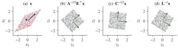
Most algorithms in this book use this reduction, from the angle search of Section 1.5第 1.5 节 to FastICA (Chapter 8第 8 章) and JADE (Chapter 9第 9 章); Comon (1994) built his ICA algorithm on it, and Hyvärinen, Karhunen and Oja (2001) give a textbook account. Figure 3.1图 3.1 shows its geometry. The reduction also has costs, which the second half of the chapter examines. When there are more sensors than sources, whitening is where the dimension is reduced and where noise enters (Section 3.6第 3.6 节). And because whitening is fixed before the rotation is estimated, its sampling error can never be corrected afterwards (Section 3.7第 3.7 节).

本书的大多数算法都采用这种约化，从Section 1.5第 1.5 节中的角度搜索，到 FastICA（Chapter 8第 8 章）和 JADE（Chapter 9第 9 章）；Comon（1994）的 ICA 算法就建立在这种约化之上，Hyvärinen、Karhunen 与 Oja（2001）的教材也有系统的介绍。Figure 3.1图 3.1 展示了它的几何含义。这种约化也有代价，本章后半部分专门讨论。当传感器多于源时，降维和噪声的引入都发生在白化这一步（Section 3.6第 3.6 节）。而且白化在估计旋转之前就已固定，它的抽样误差事后再也无法纠正（Section 3.7第 3.7 节）。

3.2 Centering and covariance中心化与协方差

Let $\bx \in \R^m$ have finite second moments. Centering replaces $\bx$ by $\bx - \E[\bx]$; in the model $\bx = \bA\bs$ this removes the source means, which can be restored at the end as $\bW\E[\bx]$ (Section 1.2第 1.2 节). From now on $\bx$ has zero mean and covariance $\bC_{\bx} = \E[\bx\bx^\top]$. Under the model, the source covariance $\bC_{\bs} = \E[\bs\bs^\top]$ is diagonal because the sources are independent, and

设 $\bx \in \R^m$ 的二阶矩有限。中心化就是用 $\bx - \E[\bx]$ 代替 $\bx$；在模型 $\bx = \bA\bs$ 中，这一步去掉了源的均值，而源的均值可以在最后用 $\bW\E[\bx]$ 恢复（Section 1.2第 1.2 节）。以下总设 $\bx$ 均值为零，协方差为 $\bC_{\bx} = \E[\bx\bx^\top]$。在模型之下，由于各源独立，源的协方差 $\bC_{\bs} = \E[\bs\bs^\top]$ 是对角的，并且

which equals $\bA\bA^\top$ for unit-variance sources. The covariance is symmetric and positive semidefinite, and its rank equals that of $\bA$, which is $n$ under Assumption 1.1假设 1.1. It is positive definite when $m = n$. When $m > n$ it is singular in the noise-free model, and its null space is the orthogonal complement of the column space of $\bA$.

对单位方差的源，它等于 $\bA\bA^\top$。协方差是对称半正定矩阵，其秩等于 $\bA$ 的秩，在Assumption 1.1假设 1.1下为 $n$。当 $m = n$ 时它正定。当 $m > n$ 时，在无噪声模型中它是奇异的，其零空间是 $\bA$ 列空间的正交补。

From samples $\bx(1), \dots, \bx(T)$, collected as the columns of $\bX \in \R^{m \times T}$, the sample mean $\bar\bx = \frac1T\sum_t \bx(t)$ and the sample covariance

给定样本 $\bx(1), \dots, \bx(T)$，并把它们排成 $\bX \in \R^{m \times T}$ 的各列，用样本均值 $\bar\bx = \frac1T\sum_t \bx(t)$ 和样本协方差

replace their population counterparts. Dividing by $T - 1$ instead of $T$ makes $\hat\bC_{\bx}$ unbiased; for ICA the choice is immaterial, since it rescales all whitened outputs by the same constant. When fourth moments are finite, each entry of $\hat\bC_{\bx}$ has a standard error of order $T^{-1/2}$, a fact that returns in Section 3.7第 3.7 节. Because the centered samples sum to zero, $\hat\bC_{\bx}$ has rank at most $T - 1$, so it is singular whenever $m \ge T$, and a reduction of dimension is then unavoidable. This is the situation in temporal ICA of fMRI, where the voxels play the role of sensors (Section 14.3第 14.3 节).

来代替相应的总体量。分母用 $T - 1$ 代替 $T$ 可使 $\hat\bC_{\bx}$ 无偏；对 ICA 而言这无关紧要，因为它只是把所有白化后的输出乘上同一个常数。当四阶矩有限时，$\hat\bC_{\bx}$ 每个元素的标准误都是 $T^{-1/2}$ 量级，这一点在Section 3.7第 3.7 节中还会用到。由于中心化后的样本之和为零，$\hat\bC_{\bx}$ 的秩至多为 $T - 1$，所以当 $m \ge T$ 时它必然奇异，此时降维不可避免。fMRI 的时间 ICA 就属于这种情形，在那里体素扮演传感器的角色（Section 14.3第 14.3 节）。

Numerically, the eigenvectors and eigenvalues of $\hat\bC_{\bx}$ are best obtained from the singular value decomposition $\tilde\bX = \mathbf{E}\boldsymbol{\Gamma}\bF^\top$: the eigenvectors are the columns of $\mathbf{E}$ and the eigenvalues are $\gamma_i^2/T$. This avoids forming $\tilde\bX\tilde\bX^\top$, which squares the condition number (Golub & Van Loan, 2013).

在数值计算上，$\hat\bC_{\bx}$ 的特征向量与特征值最好通过奇异值分解 $\tilde\bX = \mathbf{E}\boldsymbol{\Gamma}\bF^\top$ 求得：特征向量是 $\mathbf{E}$ 的各列，特征值为 $\gamma_i^2/T$。这样可以避免显式构造 $\tilde\bX\tilde\bX^\top$，后者会把条件数平方（Golub & Van Loan, 2013）。

3.3 Whitening matrices白化矩阵

A random vector is white if its components are uncorrelated and have unit variance. Whitening transforms the data linearly so that they become white.

若一个随机向量的各分量互不相关且方差为一，则称它是白的。白化就是对数据作线性变换，使之变白。

Since $\rank(\bV\bC_{\bx}\bV^\top) \le \rank\bC_{\bx}$, necessarily $k \le \rank\bC_{\bx}$. In the noise-free model $\rank\bC_{\bx} = n$, and whitening to $k = n$ components loses no information, because $\bx$ lies almost surely in the $n$-dimensional column space of $\bC_{\bx}$. Write the eigendecomposition of the covariance as $\bC_{\bx} = \mathbf{E}\bLambda\mathbf{E}^\top$, with $\mathbf{E}$ orthogonal and $\bLambda = \diag(\lambda_1, \dots, \lambda_m)$, $\lambda_1 \ge \dots \ge \lambda_m \ge 0$ (Section A.3第 A.3 节). Suppose first that $m = n$, so that all eigenvalues are positive. Three whitening matrices are in common use:

由于 $\rank(\bV\bC_{\bx}\bV^\top) \le \rank\bC_{\bx}$，必有 $k \le \rank\bC_{\bx}$。在无噪声模型中 $\rank\bC_{\bx} = n$，而白化到 $k = n$ 个分量不会丢失任何信息，因为 $\bx$ 几乎必然落在 $\bC_{\bx}$ 的 $n$ 维列空间里。把协方差的特征分解写成 $\bC_{\bx} = \mathbf{E}\bLambda\mathbf{E}^\top$，其中 $\mathbf{E}$ 正交，$\bLambda = \diag(\lambda_1, \dots, \lambda_m)$，$\lambda_1 \ge \dots \ge \lambda_m \ge 0$（Section A.3第 A.3 节）。先设 $m = n$，于是所有特征值都为正。常用的白化矩阵有三种：

• PCA whitening, $\bV = \bLambda^{-1/2}\mathbf{E}^\top$. The data are projected onto the principal axes, and each principal component is divided by its standard deviation.
• Symmetric (ZCA) whitening, $\bV = \bC_{\bx}^{-1/2} = \mathbf{E}\bLambda^{-1/2}\mathbf{E}^\top$: PCA whitening followed by the rotation $\mathbf{E}$ back to the original axes. Bell and Sejnowski (1997) named it ZCA, for zero-phase component analysis. Among all whitening matrices it changes the data least, in the sense that it minimizes $\E\|\bV\bx - \bx\|^2$ (Exercise 3.3习题 3.3; Kessy, Lewin and Strimmer (2018) discuss this and other optimality properties).
• Cholesky whitening, $\bV = \mathbf{L}^{-1}$, where $\bC_{\bx} = \mathbf{L}\mathbf{L}^\top$ with $\mathbf{L}$ lower triangular with a positive diagonal. Since $\mathbf{L}^{-1}$ is also lower triangular, $z_1$ depends only on $x_1$, $z_2$ on $x_1$ and $x_2$, and so on: Cholesky whitening is the Gram–Schmidt orthonormalization of $x_1, \dots, x_m$ in the inner product $\E[uv]$ (Exercise 3.1习题 3.1).

• PCA 白化，$\bV = \bLambda^{-1/2}\mathbf{E}^\top$。先把数据投影到主轴上，再把每个主成分除以它的标准差。
• 对称（ZCA）白化，$\bV = \bC_{\bx}^{-1/2} = \mathbf{E}\bLambda^{-1/2}\mathbf{E}^\top$：先做 PCA 白化，再用旋转 $\mathbf{E}$ 转回原来的坐标轴。Bell 与 Sejnowski（1997）称之为 ZCA，即零相位成分分析（zero-phase component analysis）。在所有白化矩阵中，它对数据的改变最小，即它使 $\E\|\bV\bx - \bx\|^2$ 最小（Exercise 3.3习题 3.3；Kessy、Lewin 与 Strimmer（2018）讨论了这一性质及其他最优性）。
• Cholesky 白化，$\bV = \mathbf{L}^{-1}$，其中 $\bC_{\bx} = \mathbf{L}\mathbf{L}^\top$，$\mathbf{L}$ 是对角元为正的下三角矩阵。由于 $\mathbf{L}^{-1}$ 也是下三角的，$z_1$ 只依赖于 $x_1$，$z_2$ 只依赖于 $x_1$ 与 $x_2$，依此类推：Cholesky 白化就是在内积 $\E[uv]$ 下对 $x_1, \dots, x_m$ 作 Gram–Schmidt 标准正交化（Exercise 3.1习题 3.1）。

Each of them satisfies $\bV\bC_{\bx}\bV^\top = \bI$; for PCA whitening, for instance, $\bLambda^{-1/2}\mathbf{E}^\top(\mathbf{E}\bLambda\mathbf{E}^\top)\mathbf{E}\bLambda^{-1/2} = \bI$. They are far from the only ones, but the set of all whitening matrices has a simple structure.

它们都满足 $\bV\bC_{\bx}\bV^\top = \bI$；以 PCA 白化为例，$\bLambda^{-1/2}\mathbf{E}^\top(\mathbf{E}\bLambda\mathbf{E}^\top)\mathbf{E}\bLambda^{-1/2} = \bI$。白化矩阵远不止这三种，但所有白化矩阵构成的集合有简单的结构。

Figure 3.1图 3.1 applies the three transforms to a mixture of two uniform sources. Each whitened cloud is a square, the image of the source square under an orthogonal matrix, and the three squares differ by rotations.

Figure 3.1图 3.1 把这三种变换用于两个均匀分布源的混合。每个白化后的点云都是一个正方形，即源所在的正方形在某个正交矩阵下的像，而三个正方形之间只差旋转。

3.4 The whitened model白化后的模型

Now apply a whitening matrix to the ICA model. If $\bV \in \R^{n \times m}$ whitens $\bx = \bA\bs$, then

现在把白化矩阵作用到 ICA 模型上。若 $\bV \in \R^{n \times m}$ 是 $\bx = \bA\bs$ 的白化矩阵，则

The whitened data follow an ICA model with the same sources and a square mixing matrix $\tilde\bA$, which turns out to be orthogonal.

白化后的数据服从一个源不变、混合矩阵为方阵 $\tilde\bA$ 的 ICA 模型，而 $\tilde\bA$ 恰好是正交的。

Three consequences follow. First, all white versions of the data differ by rotations, also when $m > n$: if $\bV_1$ and $\bV_2$ both whiten, then $\bz_k = \tilde\bA_k\bs$ with $\tilde\bA_k$ orthogonal, so $\bz_2 = \tilde\bA_2\tilde\bA_1^\top\bz_1$. Second, ICA on whitened data is a search over orthogonal matrices. An orthogonal unmixing matrix $\bU$ for $\bz$ yields the global matrix $\bP = \bU\tilde\bA$, which is again orthogonal; an orthogonal matrix of the form $\bPi\bD$ must have $\bD = \diag(\pm 1)$ (Section A.2第 A.2 节), so the separating orthogonal matrices are exactly $\bU = \bPi\bD\tilde\bA^\top$ with $\bPi\bD$ a signed permutation. (As elsewhere in the book, we loosely call such matrices rotations; strictly, those with determinant $-1$ also contain a reflection.) Whitening has fixed the scale of every output, $\E[y_i^2] = 1$, and only signs and order remain free. Third, the unmixing matrix for $\bx$ factors as

由此得到三个推论。第一，即使 $m > n$，数据的所有白化版本之间也只差旋转：若 $\bV_1$ 与 $\bV_2$ 都是白化矩阵，则 $\bz_k = \tilde\bA_k\bs$，$\tilde\bA_k$ 正交，所以 $\bz_2 = \tilde\bA_2\tilde\bA_1^\top\bz_1$。第二，对白化后的数据做 ICA，就是在正交矩阵中搜索。$\bz$ 的正交解混矩阵 $\bU$ 给出的全局矩阵 $\bP = \bU\tilde\bA$ 仍是正交的；而形如 $\bPi\bD$ 的正交矩阵必有 $\bD = \diag(\pm 1)$（Section A.2第 A.2 节），所以能实现分离的正交矩阵恰好是 $\bU = \bPi\bD\tilde\bA^\top$，其中 $\bPi\bD$ 是带符号的置换矩阵。（与全书其他地方一样，我们笼统地把这些矩阵称为旋转；严格说来，行列式为 $-1$ 的那些还包含一次反射。）白化已经固定了每个输出的尺度 $\E[y_i^2] = 1$，只剩符号与顺序未定。第三，$\bx$ 的解混矩阵可以分解为

where $O(n)$ is the group of $n \times n$ orthogonal matrices. For $m = n$, the parameter count of Section 1.4第 1.4 节 is now explicit: the $n^2$ entries of $\bW$ split into the $n(n+1)/2$ numbers fixed by the covariance through $\bV$ and the $n(n-1)/2$ parameters of $\bU$, the dimension of $O(n)$ (Section A.2第 A.2 节). That is one angle for $n = 2$, three for $n = 3$, and 45 for $n = 10$, against 100 entries of $\bW$. Second-order statistics thus do more than half of the work. What remains is a rotation, and estimating it is the task of the higher-order methods of Parts II and III.

其中 $O(n)$ 是 $n \times n$ 正交矩阵构成的群。对 $m = n$，Section 1.4第 1.4 节中的参数计数现在一目了然：$\bW$ 的 $n^2$ 个元素分成两部分，一部分是协方差通过 $\bV$ 确定的 $n(n+1)/2$ 个数，另一部分是 $\bU$ 的 $n(n-1)/2$ 个参数，即 $O(n)$ 的维数（Section A.2第 A.2 节）。$n = 2$ 时只剩一个角度，$n = 3$ 时剩三个，$n = 10$ 时剩 45 个，而 $\bW$ 有 100 个元素。可见二阶统计量完成了一多半的工作。剩下的是一个旋转，估计它是第二、三部分中高阶方法的任务。

Different whitening matrices give different, but rotation-equivalent, whitened mixing matrices. ZCA whitening gives a particularly natural one: for unit-variance sources and $m = n$, $\tilde\bA = \bC_{\bx}^{-1/2}\bA = (\bA\bA^\top)^{-1/2}\bA$ is the orthogonal factor of the polar decomposition of $\bA$, which is the orthogonal matrix closest to $\bA$ (Proposition A.4命题 A.4). When the mixing is mild, with $\bA$ close to the identity, ZCA-whitened data are therefore already nearly separated. For the $\bA$ used in Figure 3.1图 3.1, this $\tilde\bA$ is a rotation by about 6°, visible in panel (c).

不同的白化矩阵给出不同的、但彼此只差旋转的白化混合矩阵。ZCA 白化给出的那一个尤其自然：对单位方差的源且 $m = n$，$\tilde\bA = \bC_{\bx}^{-1/2}\bA = (\bA\bA^\top)^{-1/2}\bA$ 正是 $\bA$ 的极分解中的正交因子，也就是离 $\bA$ 最近的正交矩阵（Proposition A.4命题 A.4）。因此当混合较弱、$\bA$ 接近单位阵时，ZCA 白化后的数据已经接近分离。对Figure 3.1图 3.1所用的 $\bA$，这个 $\tilde\bA$ 是约 6° 的旋转，在（c）中可以看到。

Methods that estimate $\bW$ directly among all invertible matrices, such as maximum likelihood with the natural gradient (Chapter 7第 7 章), do not need this reduction, although they are often run on whitened data. What the orthogonality constraint costs is examined in Section 3.7第 3.7 节.

直接在全体可逆矩阵中估计 $\bW$ 的方法，例如用自然梯度求最大似然（Chapter 7第 7 章），并不需要这种约化，尽管实践中也常在白化后的数据上运行。正交约束的代价将在Section 3.7第 3.7 节中讨论。

3.5 Why second-order statistics cannot do more为什么二阶统计量做不到更多

After whitening, the covariance is used up. For every orthogonal $\bU$, the output $\by = \bU\bz$ is again white, $\E[\by\by^\top] = \bU\bU^\top = \bI$, so no criterion that depends on the data only through their covariance can prefer one rotation to another. To find $\bU$, ICA must use statistics of order higher than two or, if the sources are time series, their temporal structure.

白化之后，协方差已经用尽。对任意正交矩阵 $\bU$，输出 $\by = \bU\bz$ 仍然是白的，$\E[\by\by^\top] = \bU\bU^\top = \bI$；因此，任何只通过协方差依赖于数据的准则，都无法在不同旋转之间作出取舍。要找到 $\bU$，ICA 必须利用二阶以上的统计量；若源是时间序列，也可以利用它们的时间结构。

For Gaussian sources nothing else is available. If $\bs \sim \Ncal(\bzero, \bI)$, then $\bz = \tilde\bA\bs \sim \Ncal(\bzero, \bI)$ and $\by = \bU\bz \sim \Ncal(\bzero, \bI)$ for every orthogonal $\bU$ (Exercise 1.3习题 1.3). The distribution of the outputs does not depend on $\bU$ at all, so every rotation is an equally good answer, and higher-order statistics cannot help, since all cumulants of order three and higher vanish (Proposition 2.8命题 2.8).

对高斯源，除协方差之外别无可用的信息。若 $\bs \sim \Ncal(\bzero, \bI)$，则 $\bz = \tilde\bA\bs \sim \Ncal(\bzero, \bI)$，并且对任意正交矩阵 $\bU$ 都有 $\by = \bU\bz \sim \Ncal(\bzero, \bI)$（Exercise 1.3习题 1.3）。输出的分布与 $\bU$ 完全无关，每个旋转都是同样好的答案；高阶统计量也帮不上忙，因为三阶及以上的累积量全为零（Proposition 2.8命题 2.8）。

For non-Gaussian sources the higher-order cumulants are not rotation invariant. By (2.3) applied to $\bz = \tilde\bA\bs$, the kurtosis of the projection onto a unit vector $\bw$ is

对非高斯源，高阶累积量在旋转下不再不变。把 (2.3) 用于 $\bz = \tilde\bA\bs$，可得 $\bz$ 在单位向量 $\bw$ 上投影的峭度：

where $\tilde\ba_p$ is the $p$-th column of $\tilde\bA$. If some $\kappa_p \ne 0$, this function is not constant on the unit sphere: with $\bq = \tilde\bA^\top\bw$ and $\be_p$ the $p$-th coordinate vector, its values at $\bq = \be_p$ and at $\bq = (\be_p + \be_r)/\sqrt2$ are $\kappa_p$ and $(\kappa_p + \kappa_r)/4$, and these can all be equal only if every $\kappa_p$ is zero. Fourth-order statistics therefore distinguish directions, and Chapter 5第 5 章 proves that the local maxima of $|\kurt(\bw^\top\bz)|$ are exactly the directions $\pm\tilde\ba_p$ of the sources with nonzero kurtosis (Theorem 5.3定理 5.3).

其中 $\tilde\ba_p$ 是 $\tilde\bA$ 的第 $p$ 列。只要某个 $\kappa_p \ne 0$，这个函数在单位球面上就不是常数：记 $\bq = \tilde\bA^\top\bw$，$\be_p$ 为第 $p$ 个坐标向量，它在 $\bq = \be_p$ 与 $\bq = (\be_p + \be_r)/\sqrt2$ 处的值分别为 $\kappa_p$ 与 $(\kappa_p + \kappa_r)/4$，而这些值全部相等的唯一可能是所有 $\kappa_p$ 都为零。所以四阶统计量能够区分方向；Chapter 5第 5 章将证明，$|\kurt(\bw^\top\bz)|$ 的局部极大点恰好是峭度非零的那些源的方向 $\pm\tilde\ba_p$（Theorem 5.3定理 5.3）。

Between the two extremes, Chapter 4第 4 章 shows that a single Gaussian source does no harm, whereas with $k \ge 2$ Gaussian sources any rotation within the subspace they span leaves the distribution of $\bz$ unchanged, so only that subspace can be identified (Section 4.4第 4.4 节). The special role of the Gaussian is no accident: if a random vector with $n \ge 2$ independent components has a distribution that is invariant under all rotations, its components are Gaussian with a common variance (Exercise 3.5习题 3.5).

介于两种极端之间的情形，Chapter 4第 4 章证明：单个高斯源无碍大局；而当有 $k \ge 2$ 个高斯源时，在它们张成的子空间内作任意旋转都不改变 $\bz$ 的分布，所以只能辨识出这个子空间（Section 4.4第 4.4 节）。高斯分布的这种特殊地位并非偶然：若一个具有 $n \ge 2$ 个独立分量的随机向量，其分布在一切旋转下不变，则它的各分量都是方差相同的高斯变量（Exercise 3.5习题 3.5）。

Second-order statistics can do more when the samples are not i.i.d. If the sources are stationary time series, the lagged covariances of the whitened data are

当样本不再独立同分布时，二阶统计量可以做得更多。若各源是平稳时间序列，白化数据的时滞协方差为

where $\rho_i(\tau) = \E[s_i(t)\,s_i(t - \tau)]$ is the autocorrelation of source $i$. These matrices are not invariant under rotation. They determine $\tilde\bA$ up to a signed permutation as soon as, for every pair of sources, the two autocorrelation functions differ at some lag, even if all sources are Gaussian; this is the basis of AMUSE and SOBI (Chapter 9第 9 章, Theorem 9.6定理 9.6). Under the i.i.d. model of Assumption 1.1假设 1.1, however, the covariance is all that second-order statistics provide.

其中 $\rho_i(\tau) = \E[s_i(t)\,s_i(t - \tau)]$ 是源 $i$ 的自相关函数。这些矩阵在旋转下不是不变的。只要对每一对源，它们的自相关函数在某个时滞处不同，这些矩阵就能在带符号置换的意义下确定 $\tilde\bA$，即使所有源都是高斯的也是如此；这正是 AMUSE 与 SOBI 的基础（Chapter 9第 9 章，Theorem 9.6定理 9.6）。但在Assumption 1.1假设 1.1的独立同分布模型下，二阶统计量所能提供的只有协方差。

3.6 PCA dimension reductionPCA 降维

When there are more sensors than sources, $m > n$, whitening also reduces the dimension. In the noise-free model, $\bC_{\bx} = \bA\bA^\top$ has rank $n$, and its column space, the signal subspace, is the column space of $\bA$. Let $\lambda_1 \ge \dots \ge \lambda_n > 0$ be its nonzero eigenvalues, $\mathbf{E}_n \in \R^{m \times n}$ the corresponding orthonormal eigenvectors and $\bLambda_n = \diag(\lambda_1, \dots, \lambda_n)$, so that $\bC_{\bx} = \mathbf{E}_n\bLambda_n\mathbf{E}_n^\top$. Then $\bV = \bLambda_n^{-1/2}\mathbf{E}_n^\top \in \R^{n \times m}$ satisfies $\bV\bC_{\bx}\bV^\top = \bI$, and by Proposition 3.4命题 3.4 $\bV\bA$ is an $n \times n$ orthogonal matrix. The reduction discards the $m - n$ directions in which the data have no variance.

当传感器多于源（$m > n$）时，白化同时完成降维。在无噪声模型中，$\bC_{\bx} = \bA\bA^\top$ 的秩为 $n$，它的列空间即信号子空间，就是 $\bA$ 的列空间。设 $\lambda_1 \ge \dots \ge \lambda_n > 0$ 是它的非零特征值，$\mathbf{E}_n \in \R^{m \times n}$ 是相应的标准正交特征向量，$\bLambda_n = \diag(\lambda_1, \dots, \lambda_n)$，于是 $\bC_{\bx} = \mathbf{E}_n\bLambda_n\mathbf{E}_n^\top$。则 $\bV = \bLambda_n^{-1/2}\mathbf{E}_n^\top \in \R^{n \times m}$ 满足 $\bV\bC_{\bx}\bV^\top = \bI$，并且由Proposition 3.4命题 3.4，$\bV\bA$ 是 $n \times n$ 正交矩阵。降维丢掉的是数据方差为零的那 $m - n$ 个方向。

Real data contain noise, and the eigenvalues beyond the $n$-th are then no longer zero. The simplest model in which the analysis stays exact adds isotropic noise.

真实数据含有噪声，第 $n$ 个以后的特征值不再为零。能让分析保持精确的最简单模型，是加上各向同性的噪声。

PCA thus recovers the signal subspace exactly, even with noise, and discards the noise in the $m - n$ complementary directions; this is the main denoising effect of the reduction. The noise inside the signal subspace remains. Ordinary whitening then produces a whitened mixing matrix that is not quite orthogonal, so even the best rotation leaves a bias. The bias-corrected whitening of item 4 needs an estimate of $\sigma^2$, such as the average of the $m - n$ smallest eigenvalues, which is the maximum-likelihood estimate in probabilistic PCA (Tipping & Bishop, 1999). Noisy ICA is the subject of Section 11.2第 11.2 节.

可见即使有噪声，PCA 也能准确地恢复信号子空间，并丢掉其余 $m - n$ 个方向上的噪声，这是降维最主要的去噪作用。信号子空间之内的噪声则保留下来。于是普通白化给出的白化混合矩阵并不严格正交，即使找到最好的旋转也会留下偏差。第 4 条中的偏差校正白化需要估计 $\sigma^2$，例如取最小的 $m - n$ 个特征值的平均，这正是概率 PCA 中的最大似然估计（Tipping & Bishop, 1999）。含噪 ICA 将在Section 11.2第 11.2 节中讨论。

In practice $n$ is unknown and must be read off the eigenvalues of the sample covariance, where the noise eigenvalues are no longer equal. Even pure white noise spreads them out: if $m/T \to \gamma \in (0, 1]$, the eigenvalues of the sample covariance of white noise with variance $\sigma^2$ fill the interval $[\sigma^2(1 - \sqrt\gamma)^2,\ \sigma^2(1 + \sqrt\gamma)^2]$ (Marčenko & Pastur, 1967). With $m = 250$ sensors and $T = 1000$ samples, for example, the noise eigenvalues range from about $0.25\,\sigma^2$ to $2.25\,\sigma^2$, and a weak source can hide among them. Section 11.3第 11.3 节 discusses how to choose $n$. In spatial ICA of fMRI, the role of the $m$ sensors is played by the time points, and PCA reduces them to far fewer components before ICA is run (Chapter 14第 14 章).

实践中 $n$ 未知，只能从样本协方差的特征值中读出，而样本协方差的噪声特征值不再相等。即使是纯白噪声，也会使它们散开：若 $m/T \to \gamma \in (0, 1]$，方差为 $\sigma^2$ 的白噪声的样本协方差的特征值铺满区间 $[\sigma^2(1 - \sqrt\gamma)^2,\ \sigma^2(1 + \sqrt\gamma)^2]$（Marčenko & Pastur, 1967）。例如有 $m = 250$ 个传感器、$T = 1000$ 个样本时，噪声特征值大约从 $0.25\,\sigma^2$ 分布到 $2.25\,\sigma^2$，较弱的源可能淹没其中。Section 11.3第 11.3 节讨论如何选择 $n$。在 fMRI 的空间 ICA 中，扮演 $m$ 个传感器角色的是时间点，运行 ICA 之前要先用 PCA 把它们降到少得多的成分（Chapter 14第 14 章）。

3.7 Whitening with finite samples有限样本下的白化

With finite $T$, whitening uses the sample covariance. The whitened sample $\hat\bz(t) = \hat\bV\bx(t)$ is then exactly white, $\frac1T\sum_t \hat\bz(t)\hat\bz(t)^\top = \bI$ after centering, but the whitened mixing matrix $\hat\bV\bA$ is orthogonal only up to an error of order $T^{-1/2}$ (for sources with finite fourth moments). An orthogonal method estimates an orthogonal $\bU$, so its outputs $\by(t) = \bU\hat\bz(t)$ are exactly uncorrelated in the sample. The true sources are not: their sample covariance $\hat\bC_{\bs}$ differs from $\bI$ by sampling fluctuations. The constraint imposes a property that the sources do not have, and the resulting error passes into the separation, where no choice of $\bU$ can remove it. The following proposition makes this precise; the notation $O_P$ is recalled in Section A.8第 A.8 节.

当 $T$ 有限时，白化用的是样本协方差。这时白化后的样本 $\hat\bz(t) = \hat\bV\bx(t)$（中心化之后）严格满足 $\frac1T\sum_t \hat\bz(t)\hat\bz(t)^\top = \bI$，但白化后的混合矩阵 $\hat\bV\bA$ 只在 $T^{-1/2}$ 量级的误差内是正交的（对四阶矩有限的源而言）。正交方法估计的是正交矩阵 $\bU$，所以它的输出 $\by(t) = \bU\hat\bz(t)$ 在样本中严格不相关。真实的源却并非如此：它们的样本协方差 $\hat\bC_{\bs}$ 由于抽样波动而偏离 $\bI$。这个约束强加了源本身并不具备的性质，由此产生的误差进入分离结果，任何 $\bU$ 都无法消除。下面的命题把这一点说清楚；记号 $O_P$ 的含义见Section A.8第 A.8 节。