Part IV · Chapter 10第四部分 · 第 10 章

Asymptotic Performance and the Cramér–Rao Bound渐近性能与 Cramér–Rao 界

The gain matrix and interference-to-signal ratio, asymptotic variance of contrast-based estimators, the optimal nonlinearity, and the Cramér–Rao bound for ICA.

增益矩阵与干扰信号比、基于对比函数的估计量的渐近方差、最优非线性函数，以及 ICA 的 Cramér–Rao 界。

10.1 How accurate can separation be?分离能做到多精确？

An ICA algorithm computes its estimate from a finite sample, so even when the model holds exactly, each output keeps a small amount of the other sources. The script of Section 1.5第 1.5 节 printed $\bW\bA \approx \bigl(\begin{smallmatrix} 0.03 & 1.00 \\ -1.00 & 0.02 \end{smallmatrix}\bigr)$ : separation succeeded, but the entries $0.03$ and $0.02$ are not zero, and they would change with a new sample. This chapter quantifies such residual errors. How large are they? How do they depend on the sample size $T$ , on the distributions of the sources and on the algorithm? Is there a limit that no algorithm can beat?

ICA 算法的估计来自有限样本，所以即使模型完全成立，每个输出里仍会残留少量其他源的成分。Section 1.5第 1.5 节的脚本输出 $\bW\bA \approx \bigl(\begin{smallmatrix} 0.03 & 1.00 \\ -1.00 & 0.02 \end{smallmatrix}\bigr)$ ：分离成功了，但 $0.03$ 和 $0.02$ 这两个元素并不为零，换一组样本它们还会变。本章定量刻画这种残余误差：它有多大？它如何依赖于样本量 $T$ 、源的分布以及所用的算法？是否存在任何算法都无法突破的极限？

The answers are asymptotic: they describe the leading behaviour of the errors as $T \to \infty$ , and in practice they are accurate already for moderate $T$ . Three facts organize the chapter. For the usual estimators the distribution of the errors does not depend on the mixing matrix (Section 10.2第 10.2 节). The errors shrink like $1/\sqrt{T}$ , with constants that can be computed in closed form; for one-unit FastICA the constant is the asymptotic variance $V_g$ of Hyvärinen (1997; 1999), and the best nonlinearity is the score function of the source (Section 10.5第 10.5 节). Finally, the Cramér–Rao bound (Tichavský, Koldovský & Oja, 2006) gives the smallest variance that any unbiased estimator can achieve; it is governed by the Fisher information of the sources and becomes infinite when two sources are Gaussian (Section 10.7第 10.7 节).

这些答案都是渐近的：它们描述 $T \to \infty$ 时误差的主导行为，而实践中 $T$ 不太大时就已相当准确。本章围绕三个事实展开。对常用的估计量，误差的分布与混合矩阵无关（Section 10.2第 10.2 节）。误差以 $1/\sqrt{T}$ 的速度缩小，其常数可以写成闭式：对单单元 FastICA，这个常数就是 Hyvärinen（1997; 1999）给出的渐近方差 $V_g$ ，而最优的非线性函数是源的得分函数（Section 10.5第 10.5 节）。最后，Cramér–Rao 界（Tichavský, Koldovský & Oja, 2006）给出任何无偏估计量所能达到的最小方差；它由源的 Fisher 信息决定，两个源都是高斯时变为无穷大（Section 10.7第 10.7 节）。

Throughout the chapter the model is square ( $m = n$ , $\bA$ invertible), the sources satisfy Assumption 1.1假设 1.1 with zero mean and unit variance, and their densities $p_i$ are smooth enough for every expectation below to exist and for differentiation under the integral sign. The score function is $\psi_i = -p_i'/p_i$ and the Fisher information is $\mathcal{J}_i = \E[\psi_i^2(s_i)]$ (Definition 6.1定义 6.1). One identity is used repeatedly. If $f$ is differentiable and $f(s)p(s) \to 0$ as $|s| \to \infty$ , integration by parts gives $\int f'p\,ds = -\int fp'\,ds = \int f\psi p\,ds$ , that is,

本章始终假设模型为方阵（ $m = n$ ， $\bA$ 可逆），源满足Assumption 1.1假设 1.1，均值为零、方差为一，并且密度 $p_i$ 足够光滑，使下文出现的期望都存在，积分号下也可以求导。得分函数记为 $\psi_i = -p_i'/p_i$ ，Fisher 信息记为 $\mathcal{J}_i = \E[\psi_i^2(s_i)]$ （Definition 6.1定义 6.1）。有一个恒等式会反复用到：若 $f$ 可微，且 $|s| \to \infty$ 时 $f(s)p(s) \to 0$ ，则分部积分给出 $\int f'p\,ds = -\int fp'\,ds = \int f\psi p\,ds$ ，即

\E[f'(s)] = \E[\psi(s)\,f(s)].\tag{10.1}

With $f = 1$ , $f(s) = s$ and $f = \psi$ it yields $\E[\psi(s)] = 0$ , $\E[s\,\psi(s)] = 1$ and $\E[\psi'(s)] = \mathcal{J}$ . For a standard Gaussian $\psi(s) = s$ , so $\mathcal{J} = 1$ ; every other unit-variance law has $\mathcal{J} > 1$ , because $\E[(\psi(s) - s)^2] = \mathcal{J} - 2 + 1 = \mathcal{J} - 1$ vanishes only when $\psi(s) = s$ .

取 $f = 1$ 、 $f(s) = s$ 和 $f = \psi$ ，依次得到 $\E[\psi(s)] = 0$ 、 $\E[s\,\psi(s)] = 1$ 和 $\E[\psi'(s)] = \mathcal{J}$ 。标准高斯分布的 $\psi(s) = s$ ，因此 $\mathcal{J} = 1$ ；其他任何方差为一的分布都有 $\mathcal{J} > 1$ ，因为 $\E[(\psi(s) - s)^2] = \mathcal{J} - 2 + 1 = \mathcal{J} - 1$ 只在 $\psi(s) = s$ 时为零。

10.2 The gain matrix and the interference-to-signal ratio增益矩阵与干扰信号比

Let $\hat\bW$ be an estimate of the unmixing matrix computed from $T$ samples. Its quality is judged not by $\hat\bW$ itself, which depends on the arbitrary scaling of the outputs, but by what it does to the sources.

设 $\hat\bW$ 是由 $T$ 个样本算出的解混矩阵估计。评价它的好坏，不看 $\hat\bW$ 本身（它依赖于输出的任意尺度），而看它对源做了什么。

Definition 10.1 (gain matrix and its error)定义 10.1（增益矩阵及其误差）

The gain matrix of $\hat\bW$ is $\hat\bP = \hat\bW\bA$ , so that the outputs are $\hat\by = \hat\bP\bs$ . Order the outputs so that output $i$ estimates source $i$ , and let $\hat\bD = \diag(\hat P_{11}, \dots, \hat P_{nn})$ . The gain error is the matrix $\bepsilon$ with zero diagonal defined by

$\hat\bW$ 的增益矩阵是 $\hat\bP = \hat\bW\bA$ ，于是输出为 $\hat\by = \hat\bP\bs$ 。把输出排好顺序，使第 $i$ 个输出估计第 $i$ 个源，并记 $\hat\bD = \diag(\hat P_{11}, \dots, \hat P_{nn})$ 。增益误差是对角元为零的矩阵 $\bepsilon$ ，定义为

\hat\bD^{-1}\hat\bP = \bI + \bepsilon, \qquad \varepsilon_{ij} = \frac{\hat P_{ij}}{\hat P_{ii}} \quad (i \ne j).\tag{10.2}

Output $i$ is then $\hat P_{ii}\bigl(s_i + \sum_{j \ne i}\varepsilon_{ij}s_j\bigr)$ : after the unrecoverable scale $\hat P_{ii}$ has been divided out, $\varepsilon_{ij}$ is the amount of source $j$ that leaks into the estimate of source $i$ . Perfect separation means $\bepsilon = \bzero$ .

于是第 $i$ 个输出等于 $\hat P_{ii}\bigl(s_i + \sum_{j \ne i}\varepsilon_{ij}s_j\bigr)$ ：除掉无法恢复的尺度 $\hat P_{ii}$ 之后， $\varepsilon_{ij}$ 就是源 $j$ 漏进源 $i$ 的估计中的分量。完全分离意味着 $\bepsilon = \bzero$ 。

Definition 10.2 (interference-to-signal ratio)定义 10.2（干扰信号比）

The interference-to-signal ratio of source $j$ in output $i$ is $\mathrm{ISR}_{ij} = \E[\varepsilon_{ij}^2]$ , $i \ne j$ , where the expectation is over the random sample. The total ISR of output $i$ is $\sum_{j \ne i}\mathrm{ISR}_{ij}$ .

源 $j$ 在输出 $i$ 中的干扰信号比（ISR）定义为 $\mathrm{ISR}_{ij} = \E[\varepsilon_{ij}^2]$ （ $i \ne j$ ），期望对随机样本求取。输出 $i$ 的总 ISR 为 $\sum_{j \ne i}\mathrm{ISR}_{ij}$ 。

Because the sources have unit variance, $\varepsilon_{ij}^2$ is the ratio of the power that source $j$ contributes to output $i$ to the power of the wanted source in that output. ISRs are often quoted in decibels, $10\log_{10}\mathrm{ISR}$ ; the reciprocal is the signal-to-interference ratio (SIR). In a simulation $\bA$ is known, so $\bepsilon$ can be computed in every run and the ISR estimated by averaging $\varepsilon_{ij}^2$ over runs. For the estimators of this chapter, $\sqrt{T}\,\varepsilon_{ij}$ converges in distribution to a normal law with mean zero and some variance $v_{ij}$ , the asymptotic variance. As is customary, we then use $\mathrm{ISR}_{ij} \approx v_{ij}/T$ , replacing the exact mean square by its asymptotic value; Section 10.6第 10.6 节 checks this approximation numerically. The constant $v_{ij}$ measures the statistical efficiency of a method independently of $T$ .

由于源的方差为一， $\varepsilon_{ij}^2$ 就是源 $j$ 在输出 $i$ 中贡献的功率与目标源功率之比。ISR 常以分贝表示，即 $10\log_{10}\mathrm{ISR}$ ；其倒数是信干比（SIR）。做模拟时 $\bA$ 已知，因此每次运行都能算出 $\bepsilon$ ，再对多次运行的 $\varepsilon_{ij}^2$ 求平均即可估计 ISR。对本章讨论的估计量， $\sqrt{T}\,\varepsilon_{ij}$ 依分布收敛到均值为零、方差为某个 $v_{ij}$ 的正态分布， $v_{ij}$ 称为渐近方差。按惯例，我们用 $\mathrm{ISR}_{ij} \approx v_{ij}/T$ ，即以渐近值代替精确的均方；Section 10.6第 10.6 节用数值方法检验这一近似。常数 $v_{ij}$ 衡量的是方法本身的统计效率，与 $T$ 无关。

Why the mixing matrix does not matter为什么混合矩阵无关紧要

Most ICA estimators are defined by equations that involve the data only through the outputs. Maximum likelihood and Infomax solve $\hat\E[\bphi(\by)\by^\top] = \bI$ ; the fixed points of FastICA satisfy whitening and fixed-point conditions on $\by$ ; JADE optimizes cumulants of $\by$ . Such estimators are equivariant (Cardoso & Laheld, 1996; see also Proposition 7.1命题 7.1), and equivariance has a strong consequence for performance.

大多数 ICA 估计量由一组只通过输出依赖数据的方程定义。最大似然与 Infomax 求解 $\hat\E[\bphi(\by)\by^\top] = \bI$ ；FastICA 的不动点满足关于 $\by$ 的白化条件和不动点条件；JADE 优化的是 $\by$ 的累积量。这样的估计量具有等变性（Cardoso & Laheld, 1996；另见Proposition 7.1命题 7.1），而等变性对性能有一个很强的推论。

Proposition 10.3 (performance does not depend on the mixing matrix)命题 10.3（性能与混合矩阵无关）

Suppose $\hat\bW$ solves equations $\mathbf{H}(\hat\bW\bX) = \bzero$ that depend on the data matrix $\bX$ only through the outputs $\hat\bW\bX$ , and that when several solutions exist, the one returned is chosen by a rule that also depends only on the outputs. Then the gain matrix $\hat\bP = \hat\bW\bA$ obtained from $\bX = \bA\bS$ equals the estimate obtained from the sources $\bS$ themselves. In particular, the distributions of $\hat\bP$ , $\bepsilon$ and every ISR are the same for all invertible $\bA$ .

设 $\hat\bW$ 是方程 $\mathbf{H}(\hat\bW\bX) = \bzero$ 的解，这组方程只通过输出 $\hat\bW\bX$ 依赖数据矩阵 $\bX$ ；若有多个解，则返回哪一个也只由输出决定。那么由 $\bX = \bA\bS$ 得到的增益矩阵 $\hat\bP = \hat\bW\bA$ ，等于直接用源 $\bS$ 算出的估计。特别地，对所有可逆的 $\bA$ ， $\hat\bP$ 、 $\bepsilon$ 以及每个 ISR 的分布都相同。

Proof.证明

Let $\bW_{\bS}$ be the solution returned for the data $\bS$ . The matrix $\bW_{\bS}\bA^{-1}$ produces from $\bX = \bA\bS$ exactly the same outputs, $(\bW_{\bS}\bA^{-1})(\bA\bS) = \bW_{\bS}\bS$ , so it solves the equations for $\bX$ and is the one returned. Hence $\hat\bW(\bA\bS) = \hat\bW(\bS)\,\bA^{-1}$ and $\hat\bP = \hat\bW(\bS)$ , which does not involve $\bA$ .

记 $\bW_{\bS}$ 为对数据 $\bS$ 返回的解。矩阵 $\bW_{\bS}\bA^{-1}$ 作用于 $\bX = \bA\bS$ 时给出完全相同的输出， $(\bW_{\bS}\bA^{-1})(\bA\bS) = \bW_{\bS}\bS$ ，因此它是关于 $\bX$ 的方程的解，而且就是被返回的那一个。于是 $\hat\bW(\bA\bS) = \hat\bW(\bS)\,\bA^{-1}$ ，从而 $\hat\bP = \hat\bW(\bS)$ ，与 $\bA$ 无关。

Simulation studies can therefore take $\bA = \bI$ without loss of generality, and an ill-conditioned mixing matrix does not by itself make an equivariant estimator less accurate. What can depend on $\bA$ is the path of an iterative algorithm that is not itself equivariant, such as plain gradient ascent with a fixed step size, and the numerical round-off when $\bA$ is nearly singular.

因此，模拟研究可以不失一般性地取 $\bA = \bI$ ；混合矩阵病态本身也不会降低等变估计量的精度。可能依赖于 $\bA$ 的，是本身不具等变性的迭代算法的收敛路径（例如固定步长的普通梯度上升），以及 $\bA$ 接近奇异时的数值舍入误差。

10.3 Amari's performance indexAmari 性能指标

The ISR requires the outputs to be matched to the sources and the scales to be removed. Amari, Cichocki and Yang (1996) proposed a single number that needs no matching of outputs to sources. It does depend on the scales of the outputs, which are therefore normalized first (see the invariance property below). For an $n \times n$ gain matrix $\bP = (p_{ij})$ ,

计算 ISR 需要先把输出与源配对，并除去尺度。Amari、Cichocki 和 Yang（1996）提出了一个无需把输出与源配对的单一指标。不过它依赖于输出的尺度，因此要先把输出归一化（见下面的不变性）。对 $n \times n$ 的增益矩阵 $\bP = (p_{ij})$ ，定义

E(\bP) = \sum_{i=1}^n\Bigl(\sum_{j=1}^n\frac{|p_{ij}|}{\max_k|p_{ik}|} - 1\Bigr) + \sum_{j=1}^n\Bigl(\sum_{i=1}^n\frac{|p_{ij}|}{\max_k|p_{kj}|} - 1\Bigr).\tag{10.3}

Its main properties follow directly from the definition.

它的主要性质可以直接从定义得出。

Zero exactly at separation. Each bracket is a sum of ratios in $[0, 1]$ , one of which equals $1$ , so it is nonnegative and vanishes exactly when its row (or column) has a single nonzero entry. Hence $E(\bP) \ge 0$ , with equality if and only if $\bP = \bPi\bD$ as in Proposition 1.3命题 1.3.
Range. Each bracket is at most $n - 1$ , so $0 \le E(\bP) \le 2n(n-1)$ ; the normalized index $E/(2n(n-1))$ lies in $[0, 1]$ .
Invariance. $E$ is unchanged by permutations of the rows or of the columns. A row bracket is unchanged when its row is rescaled and a column bracket when its column is rescaled, but rescaling a row changes the column brackets. In practice $E$ is computed after normalizing every output to unit variance, that is, every row of $\hat\bP$ to unit Euclidean norm (the sources having unit variance).
Relation to the ISR. With the rows normalized and the outputs matched to the sources, $|\hat P_{ii}| = 1 + O(\|\bepsilon\|^2)$ and $E(\hat\bP) = 2\sum_{i \ne j}|\varepsilon_{ij}| + O(\|\bepsilon\|^2)$ . If $\sqrt{T}\,\varepsilon_{ij}$ is approximately normal, $\E|\varepsilon_{ij}| \approx \sqrt{2\,\mathrm{ISR}_{ij}/\pi}$ , so $\E[E(\hat\bP)] \approx 2\sqrt{2/\pi}\,\sum_{i \ne j}\sqrt{\mathrm{ISR}_{ij}}$ . The Amari index decreases like $1/\sqrt{T}$ , the ISR like $1/T$ : halving the index takes four times as many samples.

恰在分离时为零。每个括号都是若干个 $[0, 1]$ 中的比值之和，其中恰有一个等于 $1$ ，所以它非负，并且当且仅当该行（或该列）只有一个非零元时为零。因此 $E(\bP) \ge 0$ ，等号成立当且仅当 $\bP = \bPi\bD$ ，与Proposition 1.3命题 1.3一致。
取值范围。每个括号至多为 $n - 1$ ，所以 $0 \le E(\bP) \le 2n(n-1)$ ；归一化指标 $E/(2n(n-1))$ 落在 $[0, 1]$ 中。
不变性。对行或列作置换， $E$ 不变。某一行乘以常数时，该行的括号不变；某一列乘以常数时，该列的括号不变；但对行作缩放会改变各列的括号。实践中先把每个输出归一化为单位方差，即把 $\hat\bP$ 的每一行归一化为单位欧氏范数（源的方差为一），再计算 $E$ 。
与 ISR 的关系。行归一化且输出与源配好对之后， $|\hat P_{ii}| = 1 + O(\|\bepsilon\|^2)$ ，并且 $E(\hat\bP) = 2\sum_{i \ne j}|\varepsilon_{ij}| + O(\|\bepsilon\|^2)$ 。若 $\sqrt{T}\,\varepsilon_{ij}$ 近似服从正态分布，则 $\E|\varepsilon_{ij}| \approx \sqrt{2\,\mathrm{ISR}_{ij}/\pi}$ ，于是 $\E[E(\hat\bP)] \approx 2\sqrt{2/\pi}\,\sum_{i \ne j}\sqrt{\mathrm{ISR}_{ij}}$ 。Amari 指标以 $1/\sqrt{T}$ 的速度下降，ISR 则以 $1/T$ 的速度下降：要把指标减半，需要四倍的样本。

Example 10.4 (reading a gain matrix)例 10.4（解读一个增益矩阵）

Take the gain matrix printed in Section 1.5第 1.5 节, $\hat\bP = \bigl(\begin{smallmatrix} 0.03 & 1.00 \\ -1.00 & 0.02 \end{smallmatrix}\bigr)$ , whose rows already have norm $1.00$ to two decimals. The row brackets are $0.03$ and $0.02$ , the column brackets $0.03$ and $0.02$ , so $E(\hat\bP) = 0.10$ and the normalized index is $0.025$ . Output 1 estimates $s_2$ and output 2 estimates $s_1$ . Reordering the outputs accordingly gives $\varepsilon_{12} = 0.02/(-1.00)$ (source 2 in the estimate of source 1) and $\varepsilon_{21} = 0.03/1.00$ (source 1 in the estimate of source 2). The realized interference-to-signal ratios are $\varepsilon_{12}^2 = 4 \times 10^{-4}$ ( $-34.0$ dB) and $\varepsilon_{21}^2 = 9 \times 10^{-4}$ ( $-30.5$ dB), and indeed $2(|\varepsilon_{12}| + |\varepsilon_{21}|) = 0.10 = E(\hat\bP)$ .

取Section 1.5第 1.5 节中输出的增益矩阵 $\hat\bP = \bigl(\begin{smallmatrix} 0.03 & 1.00 \\ -1.00 & 0.02 \end{smallmatrix}\bigr)$ ，保留两位小数时它的各行范数已经是 $1.00$ 。两个行括号分别是 $0.03$ 和 $0.02$ ，两个列括号也是 $0.03$ 和 $0.02$ ，所以 $E(\hat\bP) = 0.10$ ，归一化指标为 $0.025$ 。输出 1 估计的是 $s_2$ ，输出 2 估计的是 $s_1$ 。相应地重排输出，得到 $\varepsilon_{12} = 0.02/(-1.00)$ （源 2 漏进源 1 的估计中）和 $\varepsilon_{21} = 0.03/1.00$ （源 1 漏进源 2 的估计中）。这次实现的干扰信号比为 $\varepsilon_{12}^2 = 4 \times 10^{-4}$ （ $-34.0$ dB）和 $\varepsilon_{21}^2 = 9 \times 10^{-4}$ （ $-30.5$ dB），并且确有 $2(|\varepsilon_{12}| + |\varepsilon_{21}|) = 0.10 = E(\hat\bP)$ 。

10.4 Estimating equations and asymptotic normality估计方程与渐近正态性

Most ICA estimators are solutions of estimating equations $\frac{1}{T}\sum_{t=1}^T \mathbf{F}(\bx(t); \btheta) = \bzero$ whose population version $\E[\mathbf{F}(\bx; \btheta)] = \bzero$ holds at the true parameter $\btheta_0$ ; here $\btheta$ collects the entries of $\bW$ and $\btheta_0$ is a separating matrix. The theory of such M-estimators (Section A.8第 A.8 节; van der Vaart, 1998) states that if $\btheta_0$ is an isolated root, $\mathbf{F}$ is smooth enough and $\bM = \E[\partial\mathbf{F}/\partial\btheta^\top]$ is invertible at $\btheta_0$ , then the root $\hat\btheta$ near $\btheta_0$ is consistent and

大多数 ICA 估计量都是估计方程 $\frac{1}{T}\sum_{t=1}^T \mathbf{F}(\bx(t); \btheta) = \bzero$ 的解，其总体形式 $\E[\mathbf{F}(\bx; \btheta)] = \bzero$ 在真实参数 $\btheta_0$ 处成立；这里 $\btheta$ 由 $\bW$ 的元素组成， $\btheta_0$ 是一个分离矩阵。这类 M 估计量的理论（Section A.8第 A.8 节；van der Vaart, 1998）指出：若 $\btheta_0$ 是孤立根， $\mathbf{F}$ 足够光滑，且 $\bM = \E[\partial\mathbf{F}/\partial\btheta^\top]$ 在 $\btheta_0$ 处可逆，则 $\btheta_0$ 附近的根 $\hat\btheta$ 是相合的，并且

\sqrt{T}\,(\hat\btheta - \btheta_0) \ \xrightarrow{d}\ \Ncal\bigl(\bzero,\ \bM^{-1}\bSigma\bM^{-\top}\bigr), \qquad \bSigma = \E\bigl[\mathbf{F}(\bx; \btheta_0)\,\mathbf{F}(\bx; \btheta_0)^\top\bigr].\tag{10.4}

The argument is a first-order expansion, $\bzero = \hat\E[\mathbf{F}(\bx; \hat\btheta)] \approx \hat\E[\mathbf{F}(\bx; \btheta_0)] + \bM(\hat\btheta - \btheta_0)$ , followed by the central limit theorem for $\hat\E[\mathbf{F}(\bx; \btheta_0)]$ . The errors are therefore of order $1/\sqrt{T}$ and the ISR of order $1/T$ . For ICA the expansion has a special structure: it splits into separate $2 \times 2$ problems, one for each pair of sources.

论证就是一阶展开 $\bzero = \hat\E[\mathbf{F}(\bx; \hat\btheta)] \approx \hat\E[\mathbf{F}(\bx; \btheta_0)] + \bM(\hat\btheta - \btheta_0)$ ，再对 $\hat\E[\mathbf{F}(\bx; \btheta_0)]$ 应用中心极限定理。因此误差是 $1/\sqrt{T}$ 量级，ISR 是 $1/T$ 量级。对 ICA 而言，这个展开有特殊的结构：它分解为互不相干的若干个 $2 \times 2$ 问题，每对源一个。

Proposition 10.5 (asymptotic variance of ICA estimating equations)命题 10.5（ICA 估计方程的渐近方差）

Let $\varphi_1, \dots, \varphi_n$ be differentiable nonlinearities, and let $\hat\bW$ solve

设 $\varphi_1, \dots, \varphi_n$ 是可微的非线性函数， $\hat\bW$ 满足

\hat\E[\varphi_i(y_i)\,y_j] = 0, \qquad i \ne j,\tag{10.5}

together with $n$ scale equations (for instance $\hat\E[y_i^2] = 1$ ) whose population solution is $\bP = \bI$ up to signs. Let $\mu_i = \E[s_i\varphi_i(s_i)]$ , $\rho_i = \E[\varphi_i'(s_i)]$ , $\beta_i = \E[\varphi_i^2(s_i)]$ , and assume $\rho_i\rho_j \ne \mu_i\mu_j$ for all $i \ne j$ . Then for the solution near separation, $\sqrt{T}\,\varepsilon_{ij}$ is asymptotically normal with mean zero and variance

以及 $n$ 个尺度方程（例如 $\hat\E[y_i^2] = 1$ ），且这些方程的总体解在符号意义下为 $\bP = \bI$ 。记 $\mu_i = \E[s_i\varphi_i(s_i)]$ ， $\rho_i = \E[\varphi_i'(s_i)]$ ， $\beta_i = \E[\varphi_i^2(s_i)]$ ，并假设对所有 $i \ne j$ 有 $\rho_i\rho_j \ne \mu_i\mu_j$ 。则对分离点附近的解， $\sqrt{T}\,\varepsilon_{ij}$ 渐近服从均值为零的正态分布，方差为

v_{ij} = \frac{\rho_j^2\beta_i - 2\rho_j\mu_i^2\mu_j + \mu_i^2\beta_j}{(\rho_i\rho_j - \mu_i\mu_j)^2}.\tag{10.6}

If the data are centered with the sample mean before the equations are solved, the same holds with $\beta_i$ replaced by $\Var\varphi_i(s_i) = \beta_i - (\E[\varphi_i(s_i)])^2$ for every $i$ .

若先用样本均值把数据中心化、再求解这些方程，结论不变，只需对每个 $i$ 把 $\beta_i$ 换成 $\Var\varphi_i(s_i) = \beta_i - (\E[\varphi_i(s_i)])^2$ 。

Proof.证明

Write $\hat P_{ij} = \delta_{ij} + e_{ij}$ with all $e_{ij} = O_p(T^{-1/2})$ (signs fixed). Since $\varepsilon_{ij} = e_{ij}/(1 + e_{ii}) = e_{ij} + O_p(T^{-1})$ , it suffices to study $e_{ij}$ . The outputs are $y_i = s_i + \sum_k e_{ik}s_k$ , and a Taylor expansion of $\varphi_i$ gives

把增益矩阵写成 $\hat P_{ij} = \delta_{ij} + e_{ij}$ ，其中所有 $e_{ij} = O_p(T^{-1/2})$ （符号已固定）。由于 $\varepsilon_{ij} = e_{ij}/(1 + e_{ii}) = e_{ij} + O_p(T^{-1})$ ，只需研究 $e_{ij}$ 。输出为 $y_i = s_i + \sum_k e_{ik}s_k$ ，对 $\varphi_i$ 作 Taylor 展开得

\hat\E[\varphi_i(y_i)\,y_j] = \hat\E[\varphi_i(s_i)s_j] + \sum_k e_{jk}\,\hat\E[\varphi_i(s_i)s_k] + \sum_k e_{ik}\,\hat\E[\varphi_i'(s_i)s_ks_j] + O_p(T^{-1}).

In the two sums the sample averages can be replaced by their expectations at a cost $o_p(T^{-1/2})$ . By independence and zero means, $\E[\varphi_i(s_i)s_k]$ equals $\mu_i$ for $k = i$ and $0$ otherwise, and for $j \ne i$ , $\E[\varphi_i'(s_i)s_ks_j]$ equals $\rho_i$ for $k = j$ and $0$ otherwise. With $u_{ij} = \hat\E[\varphi_i(s_i)s_j]$ , the equations for $(i, j)$ and $(j, i)$ become

两个求和中的样本平均可以换成期望，代价为 $o_p(T^{-1/2})$ 。由独立性和零均值， $\E[\varphi_i(s_i)s_k]$ 在 $k = i$ 时等于 $\mu_i$ ，否则为 $0$ ；对 $j \ne i$ ， $\E[\varphi_i'(s_i)s_ks_j]$ 在 $k = j$ 时等于 $\rho_i$ ，否则为 $0$ 。记 $u_{ij} = \hat\E[\varphi_i(s_i)s_j]$ ，关于 $(i, j)$ 和 $(j, i)$ 的两个方程化为

\begin{pmatrix} \rho_i & \mu_i \\ \mu_j & \rho_j \end{pmatrix}\begin{pmatrix} e_{ij} \\ e_{ji} \end{pmatrix} = -\begin{pmatrix} u_{ij} \\ u_{ji} \end{pmatrix} + o_p(T^{-1/2}).

The diagonal entries $e_{ii}$ do not appear, so the scale equations play no role. Solving, $e_{ij} = (\mu_iu_{ji} - \rho_ju_{ij})/(\rho_i\rho_j - \mu_i\mu_j)$ . The pair $\sqrt{T}(u_{ij}, u_{ji})$ is an average of i.i.d. zero-mean terms; by the central limit theorem it is asymptotically normal with variances $\E[\varphi_i^2(s_i)]\E[s_j^2] = \beta_i$ , $\beta_j$ and covariance $\E[\varphi_i(s_i)s_i]\,\E[\varphi_j(s_j)s_j] = \mu_i\mu_j$ . The variance of $\rho_ju_{ij} - \mu_iu_{ji}$ is then $(\rho_j^2\beta_i - 2\rho_j\mu_i^2\mu_j + \mu_i^2\beta_j)/T$ . With centering, $\bs$ is replaced by $\bs - \bar\bs$ , where $\bar\bs$ is the sample mean of the sources. To first order this only subtracts $\bar s_j\,\E[\varphi_i(s_i)]$ from $u_{ij}$ , so $\varphi_i(s_i)$ is replaced by $\varphi_i(s_i) - \E[\varphi_i(s_i)]$ in $u_{ij}$ : the variance $\beta_i$ becomes $\Var\varphi_i(s_i)$ , and the covariance $\mu_i\mu_j$ is unchanged.

对角元 $e_{ii}$ 没有出现，所以尺度方程不起作用。解得 $e_{ij} = (\mu_iu_{ji} - \rho_ju_{ij})/(\rho_i\rho_j - \mu_i\mu_j)$ 。 $\sqrt{T}(u_{ij}, u_{ji})$ 是独立同分布、均值为零的项的平均，由中心极限定理，它渐近正态，方差分别为 $\E[\varphi_i^2(s_i)]\E[s_j^2] = \beta_i$ 和 $\beta_j$ ，协方差为 $\E[\varphi_i(s_i)s_i]\,\E[\varphi_j(s_j)s_j] = \mu_i\mu_j$ 。于是 $\rho_ju_{ij} - \mu_iu_{ji}$ 的方差为 $(\rho_j^2\beta_i - 2\rho_j\mu_i^2\mu_j + \mu_i^2\beta_j)/T$ 。做中心化时，要把 $\bs$ 换成 $\bs - \bar\bs$ ，其中 $\bar\bs$ 是源的样本均值。在一阶近似下，这只是从 $u_{ij}$ 中减去 $\bar s_j\,\E[\varphi_i(s_i)]$ ，相当于把 $u_{ij}$ 中的 $\varphi_i(s_i)$ 换成 $\varphi_i(s_i) - \E[\varphi_i(s_i)]$ ：方差 $\beta_i$ 变为 $\Var\varphi_i(s_i)$ ，协方差 $\mu_i\mu_j$ 不变。

The pairs decouple: $v_{ij}$ depends only on the laws of $s_i$ and $s_j$ and on the two nonlinearities applied to them, and it does not change when $\varphi_i$ is multiplied by a constant. With the normalization $\mu_i = 1$ of Chapter 7第 7 章, the denominator is $(\rho_i\rho_j - 1)^2$ , and $\rho_i\rho_j > 1$ is condition (iii) of Theorem 7.2定理 7.2 ( $\rho_i$ is the $k_i$ of that theorem): estimating equations whose solution is close to instability have a large variance. The most important case is the true score.

各对之间互不耦合： $v_{ij}$ 只依赖于 $s_i$ 、 $s_j$ 的分布以及作用在它们上面的两个非线性函数，而且把 $\varphi_i$ 乘以常数不改变 $v_{ij}$ 。采用Chapter 7第 7 章的归一化 $\mu_i = 1$ 时，分母为 $(\rho_i\rho_j - 1)^2$ ，而 $\rho_i\rho_j > 1$ 正是Theorem 7.2定理 7.2的条件 (iii)（ $\rho_i$ 就是该定理中的 $k_i$ ）：解接近失稳的估计方程，方差也大。最重要的情形是真实的得分函数。

Corollary 10.6 (maximum likelihood with the true scores)推论 10.6（使用真实得分函数的最大似然）

If $\varphi_i = \psi_i$ for every $i$ (maximum likelihood with the true source densities), then $v_{ij} = \mathcal{J}_j/(\mathcal{J}_i\mathcal{J}_j - 1)$ for all $i \ne j$ .

若对每个 $i$ 都取 $\varphi_i = \psi_i$ （用真实源密度做最大似然），则对所有 $i \ne j$ 有 $v_{ij} = \mathcal{J}_j/(\mathcal{J}_i\mathcal{J}_j - 1)$ 。

Proof.证明

By (10.1), $\mu_i = 1$ and $\rho_i = \beta_i = \mathcal{J}_i$ . The numerator of (10.6) becomes $\mathcal{J}_j^2\mathcal{J}_i - 2\mathcal{J}_j + \mathcal{J}_j = \mathcal{J}_j(\mathcal{J}_i\mathcal{J}_j - 1)$ and the denominator $(\mathcal{J}_i\mathcal{J}_j - 1)^2$ . Since $\E[\psi_i(s_i)] = 0$ , centering does not change this value.

由 (10.1)， $\mu_i = 1$ ， $\rho_i = \beta_i = \mathcal{J}_i$ 。于是 (10.6) 的分子化为 $\mathcal{J}_j^2\mathcal{J}_i - 2\mathcal{J}_j + \mathcal{J}_j = \mathcal{J}_j(\mathcal{J}_i\mathcal{J}_j - 1)$ ，分母为 $(\mathcal{J}_i\mathcal{J}_j - 1)^2$ 。由于 $\E[\psi_i(s_i)] = 0$ ，中心化不改变这个值。

Section 10.7第 10.7 节 shows that this value is the smallest possible: maximum likelihood with the true scores is asymptotically efficient. Pham and Garat (1997) studied the asymptotic performance of this family of quasi-maximum-likelihood estimators, in which the true scores are replaced by approximations.

Section 10.7第 10.7 节将说明这个值是可能达到的最小值：用真实得分函数的最大似然是渐近有效的。Pham 和 Garat（1997）研究了这一族拟最大似然估计量（用近似函数代替真实得分函数）的渐近性能。

The price of exact decorrelation严格去相关的代价

Many algorithms whiten with the sample covariance and then rotate (symmetric FastICA, JADE). Their outputs are exactly decorrelated in the sample, $\hat\E[\hat\by\hat\by^\top] = \bI$ , and this constraint alone fixes half of the error.

许多算法先用样本协方差白化、再做旋转（对称 FastICA、JADE）。它们的输出在样本上严格去相关，即 $\hat\E[\hat\by\hat\by^\top] = \bI$ ，而仅这一约束就确定了误差的一半。

Proposition 10.7 (decorrelated outputs)命题 10.7（去相关的输出）

Suppose the outputs satisfy $\hat\E[\hat\by\hat\by^\top] = \bI$ and, after their order and signs have been fixed, $\hat\bP - \bI = O_p(T^{-1/2})$ . Then for $i \ne j$ , $\varepsilon_{ij} + \varepsilon_{ji} = -\hat\E[s_is_j] + o_p(T^{-1/2})$ , so $\sqrt{T}(\varepsilon_{ij} + \varepsilon_{ji})$ converges in distribution to $\Ncal(0, 1)$ . Consequently, if $(\sqrt{T}\varepsilon_{ij}, \sqrt{T}\varepsilon_{ji})$ converges in distribution to a limit with variances $v_{ij}$ and $v_{ji}$ , then $v_{ij} + v_{ji} \ge \frac12$ ; to first order, $\mathrm{ISR}_{ij} + \mathrm{ISR}_{ji} \ge 1/(2T)$ , whatever the source distributions and the rotation criterion.

设输出满足 $\hat\E[\hat\by\hat\by^\top] = \bI$ ，并且固定输出的顺序与符号之后 $\hat\bP - \bI = O_p(T^{-1/2})$ 。则对 $i \ne j$ 有 $\varepsilon_{ij} + \varepsilon_{ji} = -\hat\E[s_is_j] + o_p(T^{-1/2})$ ，从而 $\sqrt{T}(\varepsilon_{ij} + \varepsilon_{ji})$ 依分布收敛到 $\Ncal(0, 1)$ 。因此，若 $(\sqrt{T}\varepsilon_{ij}, \sqrt{T}\varepsilon_{ji})$ 依分布收敛到某个方差分别为 $v_{ij}$ 与 $v_{ji}$ 的极限，则 $v_{ij} + v_{ji} \ge \frac12$ ；在一阶近似下， $\mathrm{ISR}_{ij} + \mathrm{ISR}_{ji} \ge 1/(2T)$ ，无论源的分布和旋转准则如何。

Proof.证明

We have $\hat\E[\hat\by\hat\by^\top] = \hat\bP\hat\bC_{\bs}\hat\bP^\top$ with $\hat\bC_{\bs} = \hat\E[\bs\bs^\top] = \bI + \boldsymbol{\Delta}$ . For $i \ne j$ , $\Delta_{ij}$ is the average of the i.i.d. zero-mean terms $s_i(t)s_j(t)$ , whose variance is $\E[s_i^2s_j^2] = 1$ , so $\sqrt{T}\,\Delta_{ij}$ converges in distribution to $\Ncal(0, 1)$ ; by the law of large numbers $\boldsymbol{\Delta} \to \bzero$ in probability. Write $\hat\bP = (\bI + \boldsymbol{\delta})(\bI + \bepsilon)$ with $\boldsymbol{\delta} = \hat\bD - \bI$ diagonal; by hypothesis $\boldsymbol{\delta}$ and $\bepsilon$ are $O_p(T^{-1/2})$ . Expanding $(\bI + \boldsymbol{\delta})(\bI + \bepsilon)(\bI + \boldsymbol{\Delta})(\bI + \bepsilon)^\top(\bI + \boldsymbol{\delta}) = \bI$ gives $2\boldsymbol{\delta} + \bepsilon + \bepsilon^\top + \boldsymbol{\Delta} = o_p(T^{-1/2})$ , since every other term is a product of a factor of order $T^{-1/2}$ and a factor tending to zero. The off-diagonal part is the first claim. Finally, if $(\sqrt{T}\varepsilon_{ij}, \sqrt{T}\varepsilon_{ji})$ converges to $(X, Y)$ , then $X + Y \sim \Ncal(0, 1)$ , and $1 = \Var(X + Y) \le 2\Var(X) + 2\Var(Y)$ because $\Var(X + Y) + \Var(X - Y) = 2\Var(X) + 2\Var(Y)$ .

我们有 $\hat\E[\hat\by\hat\by^\top] = \hat\bP\hat\bC_{\bs}\hat\bP^\top$ ，其中 $\hat\bC_{\bs} = \hat\E[\bs\bs^\top] = \bI + \boldsymbol{\Delta}$ 。对 $i \ne j$ ， $\Delta_{ij}$ 是独立同分布、均值为零的项 $s_i(t)s_j(t)$ 的平均，这些项的方差为 $\E[s_i^2s_j^2] = 1$ ，所以 $\sqrt{T}\,\Delta_{ij}$ 依分布收敛到 $\Ncal(0, 1)$ ；由大数定律， $\boldsymbol{\Delta}$ 依概率收敛到 $\bzero$ 。把 $\hat\bP$ 写成 $(\bI + \boldsymbol{\delta})(\bI + \bepsilon)$ ，其中 $\boldsymbol{\delta} = \hat\bD - \bI$ 为对角矩阵；由假设， $\boldsymbol{\delta}$ 与 $\bepsilon$ 都是 $O_p(T^{-1/2})$ 。展开 $(\bI + \boldsymbol{\delta})(\bI + \bepsilon)(\bI + \boldsymbol{\Delta})(\bI + \bepsilon)^\top(\bI + \boldsymbol{\delta}) = \bI$ ，得 $2\boldsymbol{\delta} + \bepsilon + \bepsilon^\top + \boldsymbol{\Delta} = o_p(T^{-1/2})$ ，因为其余每一项都是一个 $T^{-1/2}$ 量级的因子与一个趋于零的因子之积。其非对角部分就是第一个结论。最后，若 $(\sqrt{T}\varepsilon_{ij}, \sqrt{T}\varepsilon_{ji})$ 依分布收敛到 $(X, Y)$ ，则 $X + Y \sim \Ncal(0, 1)$ ；又因为 $\Var(X + Y) + \Var(X - Y) = 2\Var(X) + 2\Var(Y)$ ，所以 $1 = \Var(X + Y) \le 2\Var(X) + 2\Var(Y)$ 。

Proposition 3.6命题 3.6 states the same result for whitening with the sample covariance followed by a rotation. There the error $\bepsilon = \hat\bP - \bI$ keeps its diagonal; dividing each row of $\hat\bP$ by its diagonal entry, as in (10.2), changes the off-diagonal entries only by $O_p(1/T)$ , and centering changes $\hat\bC_{\bs}$ only by $O_p(1/T)$ . The rotation step can only reduce the antisymmetric part $\varepsilon_{ij} - \varepsilon_{ji}$ ; the symmetric part is set by the sampling error of the covariance. Section 10.7第 10.7 节 shows that the best possible estimator does better than this whenever both sources are non-Gaussian.

Proposition 3.6命题 3.6对“用样本协方差白化、再做旋转”的情形给出了同样的结果。那里的误差 $\bepsilon = \hat\bP - \bI$ 保留了对角元；像 (10.2) 那样把 $\hat\bP$ 的每一行除以其对角元，只在 $O_p(1/T)$ 量级上改变非对角元，而中心化也只在 $O_p(1/T)$ 量级上改变 $\hat\bC_{\bs}$ 。旋转这一步只能减小反对称部分 $\varepsilon_{ij} - \varepsilon_{ji}$ ；对称部分由协方差的抽样误差决定。Section 10.7第 10.7 节将说明，只要两个源都非高斯，最优估计量都能做得比这更好。

10.5 One-unit estimators and the optimal nonlinearity单单元估计量与最优非线性函数

One-unit FastICA (Algorithm 8.2算法 8.2) centers the data, whitens them with the sample covariance, $\bz = \hat\bV\bx$ , and returns a unit vector $\bw$ with $\hat\E[\bz\,g(\bw^\top\bz)] = \lambda\bw$ for some scalar $\lambda$ : the Lagrange condition for an extremum of $\hat\E[G(\bw^\top\bz)]$ on the sphere, which the update (8.3) solves. Because the sources have zero mean, we first analyse the estimator without the centering step and then state what centering changes. Suppose the solution estimates source $i$ , and write $y = \bw^\top\bz = \bq^\top\bs$ with $\bq = (\hat\bV\bA)^\top\bw$ , the row of the gain matrix that produces $y$ . The gain errors of this output are $\varepsilon_k = q_k/q_i$ , $k \ne i$ .

单单元 FastICA（Algorithm 8.2算法 8.2）先把数据中心化，再用样本协方差白化， $\bz = \hat\bV\bx$ ，然后返回一个满足 $\hat\E[\bz\,g(\bw^\top\bz)] = \lambda\bw$ （ $\lambda$ 为某个标量）的单位向量 $\bw$ ：这是 $\hat\E[G(\bw^\top\bz)]$ 在球面上取极值的 Lagrange 条件，更新式 (8.3) 求解的正是它。由于源的均值为零，我们先分析不做中心化的估计量，再说明中心化带来的变化。设这个解估计的是源 $i$ ，记 $y = \bw^\top\bz = \bq^\top\bs$ ，其中 $\bq = (\hat\bV\bA)^\top\bw$ 是增益矩阵中产生 $y$ 的那一行。这个输出的增益误差为 $\varepsilon_k = q_k/q_i$ ， $k \ne i$ 。

Theorem 10.8 (asymptotic variance of one-unit estimators)定理 10.8（单单元估计量的渐近方差）

Let $g$ be differentiable, let the expectations below exist, and let $\E[s_ig(s_i) - g'(s_i)] \ne 0$ . For the solution $\bw$ of $\hat\E[\bz\,g(\bw^\top\bz)] = \lambda\bw$ , $\|\bw\| = 1$ , near the direction of source $i$ , and for every $k \ne i$ , $\sqrt{T}\,\varepsilon_k$ is asymptotically normal with mean zero and variance

设 $g$ 可微，下列期望存在，且 $\E[s_ig(s_i) - g'(s_i)] \ne 0$ 。对方程 $\hat\E[\bz\,g(\bw^\top\bz)] = \lambda\bw$ 、 $\|\bw\| = 1$ 在源 $i$ 方向附近的解 $\bw$ ，以及每个 $k \ne i$ ， $\sqrt{T}\,\varepsilon_k$ 渐近服从均值为零的正态分布，方差为

V_g = \frac{\E[g^2(s_i)] - \bigl(\E[s_i\,g(s_i)]\bigr)^2}{\bigl(\E[s_i\,g(s_i) - g'(s_i)]\bigr)^2}.\tag{10.7}

The variance depends on the distribution of $s_i$ alone: not on the other sources and, by Proposition 10.3命题 10.3, not on $\bA$ (Hyvärinen, 1997; 1999). If the data are centered with the sample mean before whitening, as in Algorithm 8.2算法 8.2, the same holds with $\E[g^2(s_i)]$ in the numerator replaced by $\Var g(s_i) = \E[g^2(s_i)] - (\E[g(s_i)])^2$ (Wei, 2015).

这个方差只依赖于 $s_i$ 的分布：与其他源无关，并且由Proposition 10.3命题 10.3，也与 $\bA$ 无关（Hyvärinen, 1997; 1999）。若像Algorithm 8.2算法 8.2那样在白化之前先用样本均值把数据中心化，结论不变，只需把分子中的 $\E[g^2(s_i)]$ 换成 $\Var g(s_i) = \E[g^2(s_i)] - (\E[g(s_i)])^2$ （Wei, 2015）。

Proof.证明

Source coordinates. With $\bM = \hat\bV\bA$ we have $\bz = \bM\bs$ and $\bM\hat\bC_{\bs}\bM^\top = \bI$ , where $\hat\bC_{\bs} = \hat\E[\bs\bs^\top]$ , because $\hat\bV$ whitens the sample. Since $\bw = \bM^{-\top}\bq$ and $\bM^{-1}\bM^{-\top} = \hat\bC_{\bs}$ , multiplying the fixed-point condition by $\bM^{-1}$ gives $\hat\E[\bs\,g(y)] = \lambda\hat\bC_{\bs}\bq = \lambda\hat\E[\bs\,y]$ , and the constraint becomes $\|\bw\|^2 = \bq^\top\hat\bC_{\bs}\bq = \hat\E[y^2] = 1$ .

源坐标。记 $\bM = \hat\bV\bA$ ，则 $\bz = \bM\bs$ ，并且由于 $\hat\bV$ 把样本白化， $\bM\hat\bC_{\bs}\bM^\top = \bI$ ，其中 $\hat\bC_{\bs} = \hat\E[\bs\bs^\top]$ 。由于 $\bw = \bM^{-\top}\bq$ 且 $\bM^{-1}\bM^{-\top} = \hat\bC_{\bs}$ ，把不动点条件左乘 $\bM^{-1}$ 得 $\hat\E[\bs\,g(y)] = \lambda\hat\bC_{\bs}\bq = \lambda\hat\E[\bs\,y]$ ，约束则化为 $\|\bw\|^2 = \bq^\top\hat\bC_{\bs}\bq = \hat\E[y^2] = 1$ 。

Expansion. Take $i = 1$ and write $\bq = (1 + \delta)\be_1 + \sum_{k \ge 2}\eta_k\be_k$ with $\delta, \eta_k = O_p(T^{-1/2})$ , so that $\varepsilon_k = \eta_k + O_p(T^{-1})$ . For $k \ge 2$ , expand both sides of the $k$ -th equation around $y = s_1$ and replace the sample averages that multiply $\delta$ or $\eta_l$ by their expectations; since $\E[s_ks_lg'(s_1)] = \delta_{kl}\E[g'(s_1)]$ for $k, l \ge 2$ and $\E[s_ks_1g'(s_1)] = 0$ ,

展开。取 $i = 1$ ，写 $\bq = (1 + \delta)\be_1 + \sum_{k \ge 2}\eta_k\be_k$ ，其中 $\delta, \eta_k = O_p(T^{-1/2})$ ，于是 $\varepsilon_k = \eta_k + O_p(T^{-1})$ 。对 $k \ge 2$ ，把第 $k$ 个方程两边在 $y = s_1$ 处展开，并把乘以 $\delta$ 或 $\eta_l$ 的样本平均换成期望；由于对 $k, l \ge 2$ 有 $\E[s_ks_lg'(s_1)] = \delta_{kl}\E[g'(s_1)]$ ，且 $\E[s_ks_1g'(s_1)] = 0$ ，得到

\begin{aligned} \hat\E[s_k\,g(y)] &= \hat\E[s_k\,g(s_1)] + \eta_k\,\E[g'(s_1)] + o_p(T^{-1/2}), \\ \hat\E[s_k\,y] &= \hat\E[s_ks_1] + \eta_k + o_p(T^{-1/2}). \end{aligned}

The first equation ( $k = 1$ ) gives $\lambda \to \mu = \E[s_1g(s_1)]$ . Substituting,

第一个方程（ $k = 1$ ）给出 $\lambda \to \mu = \E[s_1g(s_1)]$ 。代入得

\eta_k\bigl(\mu - \E[g'(s_1)]\bigr) = \hat\E\bigl[s_k\,\bigl(g(s_1) - \mu s_1\bigr)\bigr] + o_p(T^{-1/2}).

Limit. The right side is an average of i.i.d. zero-mean terms with variance $\E[s_k^2]\,\E[(g(s_1) - \mu s_1)^2] = \E[g^2(s_1)] - \mu^2$ , using $\E[s_1g(s_1)] = \mu$ and $\E[s_1^2] = 1$ . The central limit theorem and division by $\mu - \E[g'(s_1)]$ give the result.

取极限。右边是独立同分布、均值为零的项的平均，其方差为 $\E[s_k^2]\,\E[(g(s_1) - \mu s_1)^2] = \E[g^2(s_1)] - \mu^2$ ，这里用到了 $\E[s_1g(s_1)] = \mu$ 和 $\E[s_1^2] = 1$ 。由中心极限定理并除以 $\mu - \E[g'(s_1)]$ 即得结论。

Centering. If the data are centered, the argument applies with $\bs$ replaced by $\bs - \bar\bs$ , where $\bar\bs$ is the sample mean of the sources. To first order the only change is that $\hat\E[s_k\,g(s_1)]$ gains the term $-\bar s_k\,\E[g(s_1)]$ . Hence $g(s_1)$ is replaced by $g(s_1) - \E[g(s_1)]$ on the right side, and the variance becomes $\E[g^2(s_1)] - \mu^2 - (\E[g(s_1)])^2$ .

中心化。若先把数据中心化，只需把 $\bs$ 换成 $\bs - \bar\bs$ ，上述论证依然成立，其中 $\bar\bs$ 是源的样本均值。在一阶近似下，唯一的变化是 $\hat\E[s_k\,g(s_1)]$ 多出一项 $-\bar s_k\,\E[g(s_1)]$ 。于是右边的 $g(s_1)$ 换成了 $g(s_1) - \E[g(s_1)]$ ，方差变为 $\E[g^2(s_1)] - \mu^2 - (\E[g(s_1)])^2$ 。

Three features of (10.7) matter in practice. The denominator is the quantity $\E[s\,g(s) - g'(s)]$ that decides whether the source direction is an extremum of the FastICA contrast (Chapter 8第 8 章); for a Gaussian source (10.1) with $f = g$ gives $\E[s\,g(s)] = \E[g'(s)]$ , so the variance is infinite. Second, $V_g$ does not change when $g$ is multiplied by a nonzero constant or when a multiple of $s$ is added to $g$ : only the nonlinear part of $g$ matters. Third, the numerator equals $\E[(g(s) - \mu s)^2]$ , the mean square of the part of $g(s)$ that a linear regression on $s$ does not explain. With centering the regression also contains a constant, so centering never increases $V_g$ . The two versions agree when $\E[g(s)] = 0$ , as for a symmetric source and an odd $g$ ; this is the case in all other examples of this chapter, including the simulations below, which center the data. For skewed sources they can differ appreciably: for the unit-variance exponential law shifted to zero mean (density $e^{-(s+1)}$ for $s \ge -1$ ) and $g = \tanh$ , numerical quadrature gives $V_g = 3.75$ without centering and $3.14$ with it. Table 10.1表 10.1 lists $V_g$ for the three standard nonlinearities of FastICA.

(10.7) 有三个在实践中要紧的特点。其一，分母中的 $\E[s\,g(s) - g'(s)]$ 正是决定源方向是否为 FastICA 对比函数极值点的那个量（Chapter 8第 8 章）；对高斯源，在 (10.1) 中取 $f = g$ 得 $\E[s\,g(s)] = \E[g'(s)]$ ，所以方差为无穷大。其二，把 $g$ 乘以非零常数，或给 $g$ 加上 $s$ 的倍数， $V_g$ 都不变：起作用的只是 $g$ 的非线性部分。其三，分子等于 $\E[(g(s) - \mu s)^2]$ ，即 $g(s)$ 中不能由 $s$ 的线性回归解释的部分的均方。做中心化时，回归中还多了一个常数项，所以中心化绝不会增大 $V_g$ 。当 $\E[g(s)] = 0$ 时（例如源分布对称而 $g$ 为奇函数），两种情形的结果相同；本章其余的例子都属于这种情形，包括下文先做中心化的模拟。对偏斜的源，两者可能相差不小：对平移到零均值的单位方差指数分布（ $s \ge -1$ 时密度为 $e^{-(s+1)}$ ）并取 $g = \tanh$ ，数值积分给出不做中心化时 $V_g = 3.75$ ，做中心化时 $V_g = 3.14$ 。Table 10.1表 10.1列出了 FastICA 三个标准非线性函数的 $V_g$ 。

Table 10.1. Asymptotic variance

V_g

of one-unit FastICA for unit-variance sources, computed from (10.7) by numerical quadrature, and the lower bound

1/(\mathcal{J} - 1)

of Proposition 10.9命题 10.9. The hyperbolic secant density is

\frac12\operatorname{sech}(\pi s/2)

; densities of the other laws are in Table 10.2表 10.2. The uniform density has bounded support, so

\mathcal{J}

is not defined for it (see Table 10.2表 10.2).表 10.1 单位方差源下单单元 FastICA 的渐近方差

V_g

（由 (10.7) 经数值积分算得），以及Proposition 10.9命题 10.9给出的下界

1/(\mathcal{J} - 1)

。双曲正割分布的密度为

\frac12\operatorname{sech}(\pi s/2)

；其余分布的密度见Table 10.2表 10.2。均匀分布的支撑集有界，

\mathcal{J}

对它无定义（见Table 10.2表 10.2）。

Source law源的分布	$\mathcal{J}$	$g(u) = \tanh u$	$g(u) = u\,e^{-u^2/2}$	$g(u) = u^3$	$1/(\mathcal{J} - 1)$
Laplace拉普拉斯	$2$	$2.01$	$1.82$	$6.00$	$1.00$
hyperbolic secant双曲正割	$\pi^2/8 \approx 1.234$	$4.43$	$4.37$	$9.00$	$4.28$
logistic逻辑斯谛	$\pi^2/9 \approx 1.097$	$10.37$	$10.96$	$15.43$	$10.35$
uniform均匀	—	$0.69$	$0.71$	$0.43$	—

No nonlinearity in the table is best for every law, and the cubic nonlinearity of kurtosis is the best for the uniform source but the worst for the three super-Gaussian ones. What is the best possible choice for a given source?

表中没有哪个非线性函数对所有分布都最好；峭度对应的三次函数对均匀源最好，对三个超高斯分布却最差。对给定的源，最好的选择是什么？

Proposition 10.9 (the score is the optimal nonlinearity)命题 10.9（得分函数是最优非线性函数）

Let $s$ have unit variance and a density with score $\psi$ and Fisher information $1 < \mathcal{J} < \infty$ , and let $g$ satisfy the conditions of Theorem 10.8定理 10.8 together with $g(s)p(s) \to 0$ as $|s| \to \infty$ . Then

设 $s$ 方差为一，其密度的得分函数为 $\psi$ ，Fisher 信息满足 $1 < \mathcal{J} < \infty$ ；又设 $g$ 满足Theorem 10.8定理 10.8的条件，并且 $|s| \to \infty$ 时 $g(s)p(s) \to 0$ 。则

V_g \ \ge\ \frac{1}{\mathcal{J} - 1},\tag{10.8}

with equality if and only if $g(s) = a\,\psi(s) + b\,s$ for constants $a \ne 0$ and $b$ . In particular the score function itself is optimal, with $V_\psi = 1/(\mathcal{J} - 1)$ .

等号成立当且仅当 $g(s) = a\,\psi(s) + b\,s$ ，其中 $a \ne 0$ 、 $b$ 为常数。特别地，得分函数本身就是最优的，且 $V_\psi = 1/(\mathcal{J} - 1)$ 。

Proof.证明

Let $\mu = \E[s\,g(s)]$ and $h(s) = g(s) - \mu s$ , so that the numerator of (10.7) is $\E[h^2]$ . By (10.1), $\E[g'(s)] = \E[\psi(s)g(s)]$ , hence $\E[s\,g(s) - g'(s)] = \E[(s - \psi(s))\,g(s)] = \E[(s - \psi(s))\,h(s)]$ , where the last step uses $\E[(s - \psi(s))\,s] = 1 - 1 = 0$ . By the Cauchy–Schwarz inequality,

令 $\mu = \E[s\,g(s)]$ ， $h(s) = g(s) - \mu s$ ，则 (10.7) 的分子为 $\E[h^2]$ 。由 (10.1)， $\E[g'(s)] = \E[\psi(s)g(s)]$ ，因此 $\E[s\,g(s) - g'(s)] = \E[(s - \psi(s))\,g(s)] = \E[(s - \psi(s))\,h(s)]$ ，最后一步用到了 $\E[(s - \psi(s))\,s] = 1 - 1 = 0$ 。由 Cauchy–Schwarz 不等式，

\bigl(\E[(s - \psi(s))\,h(s)]\bigr)^2 \le \E\bigl[(s - \psi(s))^2\bigr]\,\E[h^2] = (\mathcal{J} - 1)\,\E[h^2],

which is (10.8). Equality holds if and only if $h$ is proportional to $s - \psi$ , that is, $g = \mu s + c\,(s - \psi)$ with $c \ne 0$ ( $c = 0$ makes $g$ linear and the denominator zero). For $g = \psi$ : $\mu = 1$ , the numerator is $\mathcal{J} - 1$ and the denominator $(1 - \mathcal{J})^2$ . With centering, the numerator is $\E[h^2]$ for $h(s) = g(s) - \mu s - \E[g(s)]$ ; since $\E[s - \psi(s)] = 0$ , the same argument gives the same bound, with equality if and only if $g(s) = a\,\psi(s) + b\,s + d$ for constants $a \ne 0$ , $b$ and $d$ , and $V_\psi$ is unchanged because $\E[\psi(s)] = 0$ .

这就是 (10.8)。等号成立当且仅当 $h$ 与 $s - \psi$ 成比例，即 $g = \mu s + c\,(s - \psi)$ 且 $c \ne 0$ （ $c = 0$ 时 $g$ 是线性的，分母为零）。当 $g = \psi$ 时， $\mu = 1$ ，分子为 $\mathcal{J} - 1$ ，分母为 $(1 - \mathcal{J})^2$ 。做中心化时，分子为 $\E[h^2]$ ，其中 $h(s) = g(s) - \mu s - \E[g(s)]$ ；由于 $\E[s - \psi(s)] = 0$ ，同样的论证给出同一个下界，等号成立当且仅当 $g(s) = a\,\psi(s) + b\,s + d$ ，其中 $a \ne 0$ 、 $b$ 、 $d$ 为常数；又因为 $\E[\psi(s)] = 0$ ， $V_\psi$ 不变。

In terms of the contrast, $g = G' = \psi$ means $G = -\log p$ up to scale and an added quadratic: the best one-unit contrast is minus the log-density of the source. The unit-variance hyperbolic secant law has score $\frac{\pi}{2}\tanh(\pi s/2)$ , so $\tanh(au)$ with $a = \pi/2$ is optimal for it; with $a = 1$ the variance is $4.43$ instead of $4.28$ . The Laplace score is $\sqrt2\,\sign(s)$ ; $\tanh(au)$ approaches it as $a$ grows, and quadrature gives $V_g = 2.01$ , $1.11$ and $1.04$ for $a = 1$ , $10$ and $30$ , approaching the bound $1$ . For the kurtosis nonlinearity $g(u) = u^3$ , (10.7) becomes $(\E[s^6] - (\E[s^4])^2)/(\E[s^4] - 3)^2$ , which involves the sixth moment; for the Laplace law it is six times the optimum. This is the asymptotic form of the robustness argument of Section 5.6第 5.6 节. Since the density is unknown in practice, the optimum is approached either by robust general-purpose choices or by choosing for each component a nonlinearity adapted to its estimated distribution, as EFICA does (Section 10.7第 10.7 节).

从对比函数的角度看， $g = G' = \psi$ 意味着在尺度和一个附加二次项的意义下 $G = -\log p$ ：最好的单单元对比函数就是源的负对数密度。单位方差双曲正割分布的得分函数为 $\frac{\pi}{2}\tanh(\pi s/2)$ ，因此对它而言取 $a = \pi/2$ 的 $\tanh(au)$ 是最优的；取 $a = 1$ 时方差为 $4.43$ ，而不是 $4.28$ 。拉普拉斯分布的得分函数为 $\sqrt2\,\sign(s)$ ， $a$ 增大时 $\tanh(au)$ 逼近它；数值积分给出 $a = 1$ 、 $10$ 、 $30$ 时 $V_g$ 分别为 $2.01$ 、 $1.11$ 和 $1.04$ ，逐渐趋于下界 $1$ 。对峭度对应的非线性函数 $g(u) = u^3$ ，(10.7) 化为 $(\E[s^6] - (\E[s^4])^2)/(\E[s^4] - 3)^2$ ，其中出现了六阶矩；对拉普拉斯分布它是最优值的六倍。这正是Section 5.6第 5.6 节中稳健性论证的渐近形式。由于实践中密度未知，要接近最优，要么采用稳健的通用选择，要么像 EFICA 那样，根据每个成分估计出的分布为它选择相应的非线性函数（Section 10.7第 10.7 节）。

10.6 Checking the theory by simulation用模拟检验理论

The script below estimates $T \cdot \mathrm{ISR}$ for one-unit FastICA on a Laplace source mixed with two uniform sources, for $g = \tanh$ and $g(u) = u^3$ , and compares it with $V_g$ computed by Monte Carlo integration. Every run draws new sources and whitens with the sample covariance; the iteration starts at the true direction, so that the run measures the accuracy of the fixed point near source 1 rather than the chance of converging to another source.

下面的脚本对一个拉普拉斯源与两个均匀源的混合运行单单元 FastICA，分别取 $g = \tanh$ 和 $g(u) = u^3$ ，估计 $T \cdot \mathrm{ISR}$ ，并与用蒙特卡洛积分算出的 $V_g$ 比较。每次运行都重新抽取源，并用样本协方差白化；迭代从真实方向出发，因此测得的是源 1 附近那个不动点的精度，而不是收敛到其他源的概率。

import numpy as np

rng = np.random.default_rng(0)
nonlin = {"tanh": (np.tanh, lambda u: 1 - np.tanh(u) ** 2),
          "pow3": (lambda u: u ** 3, lambda u: 3 * u ** 2)}
s = rng.laplace(0, 1 / np.sqrt(2), 10**7)     # unit-variance Laplace source

n, T, runs = 3, 5000, 2000
A = rng.normal(size=(n, n))
for name, (g, dg) in nonlin.items():
    # predicted asymptotic variance V_g, expectations by Monte Carlo
    Esg, Edg = np.mean(s * g(s)), np.mean(dg(s))
    V_g = (np.mean(g(s) ** 2) - Esg ** 2) / (Esg - Edg) ** 2
    eps2 = []
    for r in range(runs):
        S = np.vstack([rng.laplace(0, 1 / np.sqrt(2), T),  # target
                       rng.uniform(-np.sqrt(3), np.sqrt(3), (2, T))])
        X = A @ S
        X -= X.mean(axis=1, keepdims=True)
        d, E = np.linalg.eigh(X @ X.T / T)
        V = E @ np.diag(d ** -0.5) @ E.T            # sample whitening
        Z = V @ X
        w = np.linalg.solve((V @ A).T, np.eye(n)[0])  # start at target
        w /= np.linalg.norm(w)
        for it in range(200):                       # one-unit FastICA
            y = w @ Z
            w_new = Z @ g(y) / T - np.mean(dg(y)) * w
            w_new /= np.linalg.norm(w_new)
            done = 1 - abs(w_new @ w) < 1e-12
            w = w_new
            if done:
                break
        q = w @ V @ A                               # row of gain matrix
        eps2.extend((q[1:] / q[0]) ** 2)
    est = T * np.mean(eps2)
    se = T * np.std(eps2) / np.sqrt(len(eps2))
    print(f"{name}: predicted V_g = {V_g:.2f}, "
          f"observed T*ISR = {est:.2f} +/- {2 * se:.2f}")

The script prints

脚本输出

tanh: predicted V_g = 2.02, observed T*ISR = 2.03 +/- 0.09
pow3: predicted V_g = 6.03, observed T*ISR = 5.74 +/- 0.25

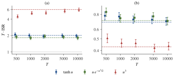
where $\pm$ is two standard errors of the Monte Carlo average (the exact values are $V_{\tanh} = 2.015$ and $V_{u^3} = 6$ ). For $\tanh$ prediction and observation agree. For $u^3$ the observed value is about $5\%$ low, just outside the Monte Carlo interval: the asymptotic formula neglects higher-order terms, and these are larger for $u^3$ , whose fluctuations are driven by high moments of the source (the denominator involves the sample kurtosis, whose variance involves $\E[s^8]$ , which equals $2520$ for the unit-variance Laplace law). Figure 10.1图 10.1 repeats the experiment over a range of $T$ and for a uniform target. All six curves settle on their predicted constants; the cubic one for the Laplace source does so only for $T$ near $10^4$ .

其中 $\pm$ 后面是蒙特卡洛平均的两倍标准误（精确值为 $V_{\tanh} = 2.015$ 和 $V_{u^3} = 6$ ）。对 $\tanh$ ，预测与观测一致。对 $u^3$ ，观测值约低 $5\%$ ，略超出蒙特卡洛区间：渐近公式忽略了高阶项，而对 $u^3$ 这些项更大，因为它的波动由源的高阶矩驱动（分母涉及样本峭度，其方差又涉及 $\E[s^8]$ ，对单位方差拉普拉斯分布这个值为 $2520$ ）。Figure 10.1图 10.1在一系列 $T$ 上重复了这一实验，并加入以均匀源为目标的情形。六条曲线都稳定到各自的预测常数上；拉普拉斯源配三次函数的那条，要到 $T$ 接近 $10^4$ 时才做到这一点。

Two panels plotting T times the ISR against the sample size T on log axes for three nonlinearities. Markers with error bars settle on dashed horizontal lines at the predicted asymptotic variances: about 2.0, 1.8 and 6 for a Laplace source in panel a, with a dotted line at the optimum 1, and about 0.69, 0.71 and 0.43 for a uniform source in panel b. — **Figure 10.1.** $T \cdot \mathrm{ISR}$ of one-unit FastICA against the sample size, for a Laplace source mixed with a uniform one (a) and a uniform source mixed with a Laplace one (b), with three nonlinearities. Markers: averages over 1500 runs with $\pm 2$ standard errors; dashed lines: $V_g$ from (10.7); dotted line in (a): the optimum $1/(\mathcal{J} - 1) = 1$ for the Laplace source.图 10.1 单单元 FastICA 的 $T \cdot \mathrm{ISR}$ 随样本量的变化：（a）拉普拉斯源与一个均匀源混合，（b）均匀源与一个拉普拉斯源混合，各用三种非线性函数。标记：1500 次运行的平均值及 $\pm 2$ 倍标准误；虚线：由 (10.7) 算出的 $V_g$ ；（a）中的点线：拉普拉斯源的最优值 $1/(\mathcal{J} - 1) = 1$ 。

10.7 The Cramér–Rao boundCramér–Rao 界

The variances computed so far belong to particular estimators. The Cramér–Rao bound limits all of them. Suppose the source densities are known, so that the unmixing matrix is the only unknown, and parametrize it around the truth as $\bW = (\bI + \mathbf{E})\bA^{-1}$ . The gain matrix is then $\bP = \bI + \mathbf{E}$ : the off-diagonal entries $E_{ij}$ are the separation errors and the diagonal entries are scale parameters. By the change of variables behind (6.1), one observation has log-density

前面算出的方差都属于具体的估计量，Cramér–Rao 界则对所有估计量都成立。假设源密度已知，唯一的未知量是解混矩阵，并在真值附近把它参数化为 $\bW = (\bI + \mathbf{E})\bA^{-1}$ 。于是增益矩阵为 $\bP = \bI + \mathbf{E}$ ：非对角元 $E_{ij}$ 就是分离误差，对角元是尺度参数。由 (6.1) 背后的变量替换，单个观测的对数密度为

\log p(\bx; \mathbf{E}) = \log|\det(\bI + \mathbf{E})| - \log|\det\bA| + \sum_{i=1}^n\log p_i(y_i), \qquad \by = (\bI + \mathbf{E})\,\bs.

Theorem 10.10 (Cramér–Rao bound for ICA)定理 10.10（ICA 的 Cramér–Rao 界）

Assume the standing assumptions, with source densities $p_i$ that are absolutely continuous and positive on $\R$ , have finite Fisher information $\mathcal{J}_i$ , and satisfy the usual regularity conditions of the Cramér–Rao inequality. At $\mathbf{E} = \bzero$ the Fisher information matrix of one observation is block diagonal: the diagonal (scale) parameters form one block, and each pair $(E_{ij}, E_{ji})$ , $i < j$ , forms the block

在本章的基本假设下，设源密度 $p_i$ 在 $\R$ 上绝对连续且处处为正，Fisher 信息 $\mathcal{J}_i$ 有限，并满足 Cramér–Rao 不等式通常的正则条件。则在 $\mathbf{E} = \bzero$ 处，单个观测的 Fisher 信息矩阵是分块对角的：对角（尺度）参数自成一块，每一对 $(E_{ij}, E_{ji})$ （ $i < j$ ）构成一块

\mathbf{F}_{ij} = \begin{pmatrix} \mathcal{J}_i & 1 \\ 1 & \mathcal{J}_j \end{pmatrix}.\tag{10.9}

If $\mathcal{J}_i\mathcal{J}_j > 1$ , every estimator $\hat{\mathbf{E}}$ that is unbiased in a neighbourhood of $\mathbf{E} = \bzero$ and uses $T$ i.i.d. observations satisfies

若 $\mathcal{J}_i\mathcal{J}_j > 1$ ，则任何在 $\mathbf{E} = \bzero$ 的某个邻域内无偏、并使用 $T$ 个独立同分布观测的估计量 $\hat{\mathbf{E}}$ 都满足

\Var(\hat E_{ij}) \ \ge\ \mathrm{CRB}(\varepsilon_{ij}) = \frac{1}{T}\,\frac{\mathcal{J}_j}{\mathcal{J}_i\mathcal{J}_j - 1}.\tag{10.10}

To first order $\hat E_{ij}$ is the gain error $\varepsilon_{ij}$ of the estimate $\hat\bW = (\bI + \hat{\mathbf{E}})\bA^{-1}$ (Tichavský, Koldovský & Oja, 2006; see also Pham & Garat, 1997).

在一阶近似下， $\hat E_{ij}$ 就是估计 $\hat\bW = (\bI + \hat{\mathbf{E}})\bA^{-1}$ 的增益误差 $\varepsilon_{ij}$ （Tichavský, Koldovský & Oja, 2006；另见 Pham & Garat, 1997）。

Proof.证明

Since $\partial\log|\det(\bI + \mathbf{E})|/\partial E_{ij} = [(\bI + \mathbf{E})^{-\top}]_{ij}$ (Section A.6第 A.6 节) and $\partial\log p_i(y_i)/\partial E_{ij} = (p_i'/p_i)(y_i)\,s_j$ , the score for $E_{ij}$ at $\mathbf{E} = \bzero$ is $\Gamma_{ij} = \delta_{ij} - \psi_i(s_i)\,s_j$ . For $i \ne j$ and $k \ne l$ , $\E[\Gamma_{ij}\Gamma_{kl}] = \E[\psi_i(s_i)s_j\,\psi_k(s_k)s_l]$ . By independence this factorizes over the sources, and any factor of the form $\E[s_l]$ or $\E[\psi_k(s_k)]$ vanishes (the latter by (10.1) with $f = 1$ ). The only nonzero cases are $(k, l) = (i, j)$ , giving $\E[\psi_i^2(s_i)]\,\E[s_j^2] = \mathcal{J}_i$ , and $(k, l) = (j, i)$ , giving $\E[\psi_i(s_i)s_i]\,\E[\psi_j(s_j)s_j] = 1$ . In the same way $\E[\Gamma_{ij}\Gamma_{kk}] = -\E[\psi_i(s_i)s_j] + \E[\psi_i(s_i)s_j\,\psi_k(s_k)s_k] = 0$ for $i \ne j$ , because every term contains $\E[s_j]$ or $\E[\psi_i(s_i)]$ . This proves the block structure. For $T$ i.i.d. observations the information is $T$ times larger, and the Cramér–Rao inequality bounds $\Var(\hat E_{ij})$ by the corresponding diagonal entry of the inverse, $[(T\mathbf{F}_{ij})^{-1}]_{11}$ , where

由于 $\partial\log|\det(\bI + \mathbf{E})|/\partial E_{ij} = [(\bI + \mathbf{E})^{-\top}]_{ij}$ （Section A.6第 A.6 节），且 $\partial\log p_i(y_i)/\partial E_{ij} = (p_i'/p_i)(y_i)\,s_j$ ，在 $\mathbf{E} = \bzero$ 处 $E_{ij}$ 的得分为 $\Gamma_{ij} = \delta_{ij} - \psi_i(s_i)\,s_j$ 。对 $i \ne j$ 、 $k \ne l$ ，有 $\E[\Gamma_{ij}\Gamma_{kl}] = \E[\psi_i(s_i)s_j\,\psi_k(s_k)s_l]$ 。由独立性，这个期望按源分解为乘积，而形如 $\E[s_l]$ 或 $\E[\psi_k(s_k)]$ 的因子都为零（后者由 (10.1) 取 $f = 1$ 得到）。只有两种情形不为零： $(k, l) = (i, j)$ 给出 $\E[\psi_i^2(s_i)]\,\E[s_j^2] = \mathcal{J}_i$ ， $(k, l) = (j, i)$ 给出 $\E[\psi_i(s_i)s_i]\,\E[\psi_j(s_j)s_j] = 1$ 。同理，对 $i \ne j$ 有 $\E[\Gamma_{ij}\Gamma_{kk}] = -\E[\psi_i(s_i)s_j] + \E[\psi_i(s_i)s_j\,\psi_k(s_k)s_k] = 0$ ，因为每一项都含有 $\E[s_j]$ 或 $\E[\psi_i(s_i)]$ 。分块结构由此得证。 $T$ 个独立同分布观测的信息量是单个观测的 $T$ 倍，Cramér–Rao 不等式用逆矩阵的相应对角元 $[(T\mathbf{F}_{ij})^{-1}]_{11}$ 给出 $\Var(\hat E_{ij})$ 的下界，其中

\mathbf{F}_{ij}^{-1} = \frac{1}{\mathcal{J}_i\mathcal{J}_j - 1}\begin{pmatrix} \mathcal{J}_j & -1 \\ -1 & \mathcal{J}_i \end{pmatrix}.

Finally $\varepsilon_{ij} = \hat E_{ij}/(1 + \hat E_{ii})$ agrees with $\hat E_{ij}$ to first order.

最后， $\varepsilon_{ij} = \hat E_{ij}/(1 + \hat E_{ii})$ 在一阶近似下与 $\hat E_{ij}$ 相同。

Practical estimators are biased at finite $T$ , so the bound is used in its asymptotic sense: under standard regularity conditions, no regular estimator that is consistent and asymptotically normal has an asymptotic variance $v_{ij}$ below $\mathcal{J}_j/(\mathcal{J}_i\mathcal{J}_j - 1)$ (van der Vaart, 1998). Comparing (10.10) with Corollary 10.6推论 10.6 shows that maximum likelihood with the true scores attains the bound.

实际的估计量在有限 $T$ 下是有偏的，因此这个界按渐近意义使用：在标准的正则条件下，任何相合且渐近正态的正则估计量，其渐近方差 $v_{ij}$ 都不会低于 $\mathcal{J}_j/(\mathcal{J}_i\mathcal{J}_j - 1)$ （van der Vaart, 1998）。把 (10.10) 与Corollary 10.6推论 10.6比较可知，用真实得分函数的最大似然达到了这个界。

What the bound says这个界说明了什么

Two Gaussian sources. If $\mathcal{J}_i = \mathcal{J}_j = 1$ , the block (10.9) is singular and the bound is infinite: the data carry no information about the rotation within the pair, as Section 4.4第 4.4 节 shows from the identifiability side.
One Gaussian source. If $\mathcal{J}_j = 1 < \mathcal{J}_i$ , then $\mathrm{CRB}(\varepsilon_{ij}) = 1/(T(\mathcal{J}_i - 1))$ but $\mathrm{CRB}(\varepsilon_{ji}) = \mathcal{J}_i/(T(\mathcal{J}_i - 1)) > 1/T$ . The non-Gaussian source is located by its non-Gaussianity; the Gaussian output can only be found as the direction uncorrelated with it, and it inherits the sampling error of the covariance (Exercise 10.4习题 10.4).
Nearly Gaussian sources. For two sources with the same law the bound is $\mathcal{J}/(T(\mathcal{J}^2 - 1))$ . With $T = 1000$ it is $6.7 \times 10^{-4}$ ( $-31.8$ dB) for Laplace sources ( $\mathcal{J} = 2$ ) but $5.4 \times 10^{-3}$ ( $-22.7$ dB) for logistic sources ( $\mathcal{J} \approx 1.097$ ): identifiable is not the same as easy to estimate (Chapter 4第 4 章).
Strongly non-Gaussian sources. As $\mathcal{J}_j \to \infty$ , $\mathrm{CRB}(\varepsilon_{ij}) \to 1/(T\mathcal{J}_i)$ and $\mathrm{CRB}(\varepsilon_{ji}) \to 0$ .
Bounded sources. A uniform density jumps at the ends of its support, the regularity conditions fail, and the bound is not defined (Tichavský et al., 2006). Smooth densities that approach the uniform law, such as the generalized Gaussian with large exponent in Table 10.2表 10.2, have $\mathcal{J} \to \infty$ , which correctly suggests that such sources are easy to separate.

两个高斯源。若 $\mathcal{J}_i = \mathcal{J}_j = 1$ ，则分块 (10.9) 奇异，界为无穷大：数据中没有关于这一对源内部旋转的任何信息，这与Section 4.4第 4.4 节从可辨识性角度得到的结论一致。
一个高斯源。若 $\mathcal{J}_j = 1 < \mathcal{J}_i$ ，则 $\mathrm{CRB}(\varepsilon_{ij}) = 1/(T(\mathcal{J}_i - 1))$ ，但 $\mathrm{CRB}(\varepsilon_{ji}) = \mathcal{J}_i/(T(\mathcal{J}_i - 1)) > 1/T$ 。非高斯源靠它的非高斯性定位；高斯输出只能作为与之不相关的方向来确定，因而继承了协方差的抽样误差（Exercise 10.4习题 10.4）。
接近高斯的源。对同分布的两个源，界为 $\mathcal{J}/(T(\mathcal{J}^2 - 1))$ 。取 $T = 1000$ ，拉普拉斯源（ $\mathcal{J} = 2$ ）的界为 $6.7 \times 10^{-4}$ （ $-31.8$ dB），逻辑斯谛源（ $\mathcal{J} \approx 1.097$ ）的界却是 $5.4 \times 10^{-3}$ （ $-22.7$ dB）：可辨识并不等于容易估计（Chapter 4第 4 章）。
强非高斯的源。当 $\mathcal{J}_j \to \infty$ 时， $\mathrm{CRB}(\varepsilon_{ij}) \to 1/(T\mathcal{J}_i)$ ，而 $\mathrm{CRB}(\varepsilon_{ji}) \to 0$ 。
有界的源。均匀分布的密度在支撑集端点处跳跃，正则条件不成立，这个界没有定义（Tichavský et al., 2006）。逼近均匀分布的光滑密度（例如Table 10.2表 10.2中指数很大的广义高斯分布）的 $\mathcal{J} \to \infty$ ，这正确地提示了这类源很容易分离。

Table 10.2. Fisher information

\mathcal{J} = \E[\psi^2(s)]

of unit-variance laws (values checked by numerical quadrature). For the generalized Gaussian law,

\beta = \sqrt{\Gamma(1/\alpha)/\Gamma(3/\alpha)}

;

\mathcal{J}

is infinite for

\alpha \le 1/2

and grows like

\alpha/3

\alpha \to \infty

. In this chapter

\nu

denotes the degrees of freedom of the Student law, not the Gaussian variable of Table 1.1表 1.1.表 10.2 单位方差分布的 Fisher 信息

\mathcal{J} = \E[\psi^2(s)]

（数值均经数值积分核对）。广义高斯分布中

\beta = \sqrt{\Gamma(1/\alpha)/\Gamma(3/\alpha)}

；

\alpha \le 1/2

时

\mathcal{J}

为无穷大，

\alpha \to \infty

时

\mathcal{J}

像

\alpha/3

一样增长。本章中

\nu

表示 Student 分布的自由度，而不是Table 1.1表 1.1中的高斯变量。

Law分布	Density密度	$\mathcal{J}$
Gaussian高斯	$\frac{1}{\sqrt{2\pi}}\,e^{-s^2/2}$	$1$
Laplace拉普拉斯	$\frac{1}{\sqrt2}\,e^{-\sqrt2\|s\|}$	$2$
logistic逻辑斯谛	$\frac{\pi}{4\sqrt3}\operatorname{sech}^2\frac{\pi s}{2\sqrt3}$	$\pi^2/9 \approx 1.097$
hyperbolic secant双曲正割	$\frac12\operatorname{sech}\frac{\pi s}{2}$	$\pi^2/8 \approx 1.234$
Student $t_\nu$ , $\nu > 2$ Student $t_\nu$ ， $\nu > 2$	$\propto \bigl(1 + \frac{s^2}{\nu - 2}\bigr)^{-(\nu+1)/2}$	$\frac{\nu(\nu+1)}{(\nu-2)(\nu+3)}$ ; $1.25$ for $\nu = 5$ $\frac{\nu(\nu+1)}{(\nu-2)(\nu+3)}$ ； $\nu = 5$ 时为 $1.25$
generalized Gaussian, $\alpha > 1/2$ 广义高斯， $\alpha > 1/2$	$\propto e^{-\|s/\beta\|^\alpha}$	$\frac{\alpha^2\,\Gamma(2 - 1/\alpha)\,\Gamma(3/\alpha)}{\Gamma(1/\alpha)^2}$ ; $1.37$ for $\alpha = 4$ $\frac{\alpha^2\,\Gamma(2 - 1/\alpha)\,\Gamma(3/\alpha)}{\Gamma(1/\alpha)^2}$ ； $\alpha = 4$ 时为 $1.37$
uniform均匀	$\frac{1}{2\sqrt3}$ on $[-\sqrt3, \sqrt3]$ 在 $[-\sqrt3, \sqrt3]$ 上为 $\frac{1}{2\sqrt3}$	not defined无定义

Which estimators attain the bound?哪些估计量能达到这个界？

Maximum likelihood with the true scores does (Corollary 10.6推论 10.6). The densities are unknown in practice, but each off-diagonal score $\psi_i(s_i)s_j$ is uncorrelated with every zero-mean function of a single source, so perturbing the marginal densities carries no first-order information about $E_{ij}$ ; this is why the same bound remains the benchmark when the densities must be learned from the data (see Amari & Cardoso, 1997, for the semiparametric theory of ICA estimating functions). Other estimators fall short of the bound, for reasons that can be identified.

用真实得分函数的最大似然可以达到（Corollary 10.6推论 10.6）。实践中密度是未知的；但每个非对角得分 $\psi_i(s_i)s_j$ 都与任何只依赖单个源的零均值函数不相关，因此扰动边缘密度不会带来关于 $E_{ij}$ 的一阶信息；这就是为什么密度需要从数据中学习时，这个界仍然是衡量标准（ICA 估计函数的半参数理论见 Amari & Cardoso, 1997）。其他估计量达不到这个界，而原因都可以说清楚。

Corollary 10.11 (one-unit estimators and the bound)推论 10.11（单单元估计量与这个界）

For $k \ne i$ , the optimal one-unit variance and the bound satisfy $\dfrac{1}{\mathcal{J}_i - 1} \ge \dfrac{\mathcal{J}_k}{\mathcal{J}_i\mathcal{J}_k - 1}$ , with equality if and only if $\mathcal{J}_k = 1$ .

对 $k \ne i$ ，单单元估计量的最优方差与这个界满足 $\dfrac{1}{\mathcal{J}_i - 1} \ge \dfrac{\mathcal{J}_k}{\mathcal{J}_i\mathcal{J}_k - 1}$ ，等号成立当且仅当 $\mathcal{J}_k = 1$ 。

Proof.证明

Both denominators are positive, and cross-multiplying gives $\mathcal{J}_i\mathcal{J}_k - 1 \ge \mathcal{J}_k(\mathcal{J}_i - 1)$ , that is, $\mathcal{J}_k \ge 1$ , with equality exactly when $\mathcal{J}_k = 1$ .

两个分母都为正，交叉相乘得 $\mathcal{J}_i\mathcal{J}_k - 1 \ge \mathcal{J}_k(\mathcal{J}_i - 1)$ ，即 $\mathcal{J}_k \ge 1$ ，等号恰在 $\mathcal{J}_k = 1$ 时成立。

A one-unit contrast looks only at the distribution of its own output and ignores the non-Gaussianity of the interfering sources, which maximum likelihood exploits. Estimators with exactly decorrelated outputs pay a different price. By Proposition 10.7命题 10.7, $\sqrt{T}(\varepsilon_{ij} + \varepsilon_{ji})$ is asymptotically $\Ncal(0, 1)$ , so to first order the sum has variance $1/T$ , while the bound for the variance of the sum, $(1, 1)\,\mathbf{F}_{ij}^{-1}(1, 1)^\top/T$ , equals

单单元对比函数只看自身输出的分布，忽略了干扰源的非高斯性，而最大似然利用了它。输出严格去相关的估计量付出的是另一种代价。由Proposition 10.7命题 10.7， $\sqrt{T}(\varepsilon_{ij} + \varepsilon_{ji})$ 渐近服从 $\Ncal(0, 1)$ ，所以在一阶近似下这个和的方差为 $1/T$ ，而这个和的方差的界 $(1, 1)\,\mathbf{F}_{ij}^{-1}(1, 1)^\top/T$ 等于

\frac{1}{T}\,\frac{\mathcal{J}_i + \mathcal{J}_j - 2}{\mathcal{J}_i\mathcal{J}_j - 1} \ \le\ \frac{1}{T},

since the difference of the two sides is proportional to $(\mathcal{J}_i - 1)(\mathcal{J}_j - 1) \ge 0$ , with equality only when one of the sources is Gaussian. Hence no estimator with exactly decorrelated outputs is asymptotically efficient for a pair of non-Gaussian sources; this limitation of prewhitened (orthogonal) methods was analysed by Cardoso (1994). Symmetric FastICA (Algorithm 8.6算法 8.6) has both limitations, since it applies one nonlinearity $g$ to all outputs and decorrelates them exactly. Tichavský, Koldovský and Oja (2006) derived its asymptotic accuracy (the result is restated as eq. (10) of Koldovský, Tichavský & Oja, 2006): for $k \ne l$ ,

因为两边之差与 $(\mathcal{J}_i - 1)(\mathcal{J}_j - 1) \ge 0$ 成正比，只有当其中一个源是高斯时才取等号。因此，对一对非高斯源，输出严格去相关的估计量都不是渐近有效的；Cardoso（1994）分析过预白化（正交）方法的这一局限。对称 FastICA（Algorithm 8.6算法 8.6）同时具有这两种局限：它对所有输出使用同一个非线性函数 $g$ ，并使输出严格去相关。Tichavský、Koldovský 和 Oja（2006）推导了它的渐近精度（Koldovský, Tichavský & Oja, 2006 的式 (10) 重述了这一结果）：对 $k \ne l$ ，

T\cdot\mathrm{ISR}_{kl} \ \to\ \frac{\gamma_k + \gamma_l + \tau_l^2}{(\tau_k + \tau_l)^2}, \qquad \gamma_k = \beta_k - \mu_k^2, \quad \tau_k = |\mu_k - \rho_k|,\tag{10.11}

with $\mu_k = \E[s_kg(s_k)]$ , $\rho_k = \E[g'(s_k)]$ and $\beta_k = \E[g^2(s_k)]$ . For two Laplace sources and $g = \tanh$ this is $1.26$ , compared with $2.01$ for the one-unit estimator and the bound $0.67$ . Exercise 10.5习题 10.5 derives (10.11) by linearizing the fixed-point conditions in the way of Proposition 10.5命题 10.5. Like (10.7), it assumes that the data are not centered with the sample mean, or that $\E[g(s_k)] = \E[g(s_l)] = 0$ ; with centering, its numerator loses $(\E[g(s_k)])^2 + (\E[g(s_l)])^2$ (Wei, 2015). EFICA (Koldovský, Tichavský & Oja, 2006) is designed to remove both limitations: it starts from symmetric FastICA, chooses for each component a nonlinearity adapted to its estimated distribution, and refines the estimate. Its authors proved that it is asymptotically efficient, attaining the Cramér–Rao bound, for generalized Gaussian sources with $\alpha > 2$ , for which the nonlinearity it selects is the score function of the source, with the exponent estimated from the data. For super-Gaussian generalized Gaussian sources with $1 \le \alpha < 2$ its accuracy is close to the bound without attaining it, and for smaller $\alpha$ it is no longer close.

其中 $\mu_k = \E[s_kg(s_k)]$ ， $\rho_k = \E[g'(s_k)]$ ， $\beta_k = \E[g^2(s_k)]$ 。对两个拉普拉斯源并取 $g = \tanh$ ，该值为 $1.26$ ，而单单元估计量为 $2.01$ ，界为 $0.67$ 。Exercise 10.5习题 10.5按Proposition 10.5命题 10.5的方式把不动点条件线性化，推导出了 (10.11)。与 (10.7) 一样，它假设数据没有按样本均值中心化，或者 $\E[g(s_k)] = \E[g(s_l)] = 0$ ；做中心化时，其分子要减去 $(\E[g(s_k)])^2 + (\E[g(s_l)])^2$ （Wei, 2015）。EFICA（Koldovský, Tichavský & Oja, 2006）旨在消除这两种局限：它从对称 FastICA 出发，根据每个成分估计出的分布为它选择相应的非线性函数，再对估计作精化。作者证明，对 $\alpha > 2$ 的广义高斯源，EFICA 选出的非线性函数就是源的得分函数（其中的指数由数据估计），因而它渐近有效、达到 Cramér–Rao 界。对 $1 \le \alpha < 2$ 的超高斯广义高斯源，其精度接近这个界但达不到它； $\alpha$ 更小时则已不再接近。

Key points

本章要点

The gain error $\varepsilon_{ij} = \hat P_{ij}/\hat P_{ii}$ measures how much of source $j$ leaks into the estimate of source $i$ ; $\mathrm{ISR}_{ij} = \E[\varepsilon_{ij}^2]$ . Once the outputs are normalized, Amari's index summarizes $\hat\bP$ without matching outputs to sources; it decreases like $1/\sqrt{T}$ .
For equivariant estimators the distribution of the errors does not depend on the mixing matrix, only on the sources and the method.
Estimators defined by estimating equations have errors of order $1/\sqrt{T}$ ; for ICA the asymptotic variance decouples into pairs of sources, and exact decorrelation makes $\sqrt{T}(\varepsilon_{ij} + \varepsilon_{ji})$ asymptotically $\Ncal(0, 1)$ .
One-unit FastICA has asymptotic variance $V_g$ , which depends only on the estimated source (and, for skewed sources, on whether the data are centered); it is minimized by the score function, with value $1/(\mathcal{J} - 1)$ .
The Cramér–Rao bound is $\mathcal{J}_j/(T(\mathcal{J}_i\mathcal{J}_j - 1))$ : infinite for two Gaussian sources, large for nearly Gaussian ones, attained by maximum likelihood with the true scores, and in general not attained by one-unit or exactly decorrelating estimators.

增益误差 $\varepsilon_{ij} = \hat P_{ij}/\hat P_{ii}$ 衡量源 $j$ 漏进源 $i$ 的估计中的多少； $\mathrm{ISR}_{ij} = \E[\varepsilon_{ij}^2]$ 。把输出归一化之后，Amari 指标无需把输出与源配对就能概括 $\hat\bP$ ，并以 $1/\sqrt{T}$ 的速度下降。
对等变估计量，误差的分布与混合矩阵无关，只取决于源和方法。
由估计方程定义的估计量误差为 $1/\sqrt{T}$ 量级；在 ICA 中渐近方差按源的两两配对解耦，而严格去相关使 $\sqrt{T}(\varepsilon_{ij} + \varepsilon_{ji})$ 渐近服从 $\Ncal(0, 1)$ 。
单单元 FastICA 的渐近方差为 $V_g$ ，它只依赖于被估计的源（对偏斜的源，还取决于数据是否做了中心化）；得分函数使它达到最小值 $1/(\mathcal{J} - 1)$ 。
Cramér–Rao 界为 $\mathcal{J}_j/(T(\mathcal{J}_i\mathcal{J}_j - 1))$ ：两个源都是高斯时为无穷大，源接近高斯时很大；用真实得分函数的最大似然可以达到它，单单元估计量和严格去相关的估计量一般达不到。

10.8 Exercises习题

Exercise 10.1习题 10.1 basic基础

Let $\hat\bP = \bigl(\begin{smallmatrix} 0.1 & 2.0 \\ -1.0 & 0.05 \end{smallmatrix}\bigr)$ . (a) Compute the Amari index $E(\hat\bP)$ . (b) Multiply the first row by $10$ and compute it again. (c) Normalize the rows to unit norm, match the outputs to the sources, and compute the gain errors, their squares in decibels, and $2\sum_{i \ne j}|\varepsilon_{ij}|$ .

设 $\hat\bP = \bigl(\begin{smallmatrix} 0.1 & 2.0 \\ -1.0 & 0.05 \end{smallmatrix}\bigr)$ 。（a）计算 Amari 指标 $E(\hat\bP)$ 。（b）把第一行乘以 $10$ 后再算一次。（c）把各行归一化为单位范数，把输出与源配对，计算增益误差、其平方的分贝值，以及 $2\sum_{i \ne j}|\varepsilon_{ij}|$ 。

Show solution查看解答

(a) Row brackets: $(0.1 + 2.0)/2.0 - 1 = 0.05$ and $(1.0 + 0.05)/1.0 - 1 = 0.05$ . Column brackets: $(0.1 + 1.0)/1.0 - 1 = 0.10$ and $(2.0 + 0.05)/2.0 - 1 = 0.025$ . Hence $E = 0.225$ . (b) The first row becomes $(1, 20)$ ; its bracket is still $0.05$ , but the columns $(1, -1)$ and $(20, 0.05)$ give brackets $1$ and $0.0025$ , so $E = 1.1025$ , although the separation is unchanged: the index is not invariant under rescaling of rows. (c) After normalization the rows are approximately $(0.050, 0.999)$ and $(-0.999, 0.050)$ . Output 1 estimates $s_2$ with $\varepsilon_{21} = 0.1/2.0 = 0.05$ , and output 2 estimates $s_1$ with $\varepsilon_{12} = 0.05/(-1.0) = -0.05$ . Both realized ISRs are $2.5 \times 10^{-3}$ , that is, $-26.0$ dB. All four brackets now equal $0.05$ , so $E = 0.20 = 2(|\varepsilon_{12}| + |\varepsilon_{21}|)$ .

（a）行括号： $(0.1 + 2.0)/2.0 - 1 = 0.05$ 和 $(1.0 + 0.05)/1.0 - 1 = 0.05$ 。列括号： $(0.1 + 1.0)/1.0 - 1 = 0.10$ 和 $(2.0 + 0.05)/2.0 - 1 = 0.025$ 。故 $E = 0.225$ 。（b）第一行变为 $(1, 20)$ ，它的括号仍是 $0.05$ ；但两列 $(1, -1)$ 和 $(20, 0.05)$ 的括号变为 $1$ 和 $0.0025$ ，于是 $E = 1.1025$ ，而分离效果并没有变：这个指标对行的缩放不具有不变性。（c）归一化后两行约为 $(0.050, 0.999)$ 和 $(-0.999, 0.050)$ 。输出 1 估计 $s_2$ ， $\varepsilon_{21} = 0.1/2.0 = 0.05$ ；输出 2 估计 $s_1$ ， $\varepsilon_{12} = 0.05/(-1.0) = -0.05$ 。两次实现的 ISR 都是 $2.5 \times 10^{-3}$ ，即 $-26.0$ dB。此时四个括号都等于 $0.05$ ，所以 $E = 0.20 = 2(|\varepsilon_{12}| + |\varepsilon_{21}|)$ 。

Exercise 10.2习题 10.2 basic基础

Show that the unit-variance Laplace density $\frac{1}{\sqrt2}e^{-\sqrt2|s|}$ has Fisher information $\mathcal{J} = 2$ . For two Laplace sources and $T = 1000$ , compute the Cramér–Rao bound for $\varepsilon_{12}$ in decibels, and compare it with one-unit FastICA using the score and using $g = \tanh$ (Table 10.1表 10.1).

证明单位方差拉普拉斯密度 $\frac{1}{\sqrt2}e^{-\sqrt2|s|}$ 的 Fisher 信息为 $\mathcal{J} = 2$ 。对两个拉普拉斯源且 $T = 1000$ ，以分贝计算 $\varepsilon_{12}$ 的 Cramér–Rao 界，并与使用得分函数和使用 $g = \tanh$ 的单单元 FastICA 比较（Table 10.1表 10.1）。

Show solution查看解答

For $s \ne 0$ , $\log p(s) = -\tfrac12\log 2 - \sqrt2|s|$ , so $\psi(s) = \sqrt2\,\sign(s)$ and $\psi^2 = 2$ almost everywhere; hence $\mathcal{J} = 2$ . The bound is $\frac{1}{T}\cdot\frac{2}{4 - 1} = \frac{2}{3T} = 6.7 \times 10^{-4}$ , or $-31.8$ dB. The one-unit estimator with the score has $1/(\mathcal{J} - 1) = 1$ , giving $10^{-3}$ ( $-30.0$ dB); with $\tanh$ , $2.015/T = 2.0 \times 10^{-3}$ ( $-27.0$ dB). The gap between the first two numbers is the information in the non-Gaussianity of the interfering source, which a one-unit contrast ignores (Corollary 10.11推论 10.11).

对 $s \ne 0$ ， $\log p(s) = -\tfrac12\log 2 - \sqrt2|s|$ ，故 $\psi(s) = \sqrt2\,\sign(s)$ ，几乎处处有 $\psi^2 = 2$ ，从而 $\mathcal{J} = 2$ 。界为 $\frac{1}{T}\cdot\frac{2}{4 - 1} = \frac{2}{3T} = 6.7 \times 10^{-4}$ ，即 $-31.8$ dB。使用得分函数的单单元估计量方差为 $1/(\mathcal{J} - 1) = 1$ ，对应 $10^{-3}$ （ $-30.0$ dB）；使用 $\tanh$ 时为 $2.015/T = 2.0 \times 10^{-3}$ （ $-27.0$ dB）。前两个数的差距，正是干扰源的非高斯性所含的信息，而单单元对比函数忽略了它（Corollary 10.11推论 10.11）。

Exercise 10.3习题 10.3 intermediate进阶

Show that for $g(u) = u^3$ the asymptotic variance (10.7) equals $(\E[s^6] - (\E[s^4])^2)/(\E[s^4] - 3)^2$ . Evaluate it for the unit-variance Laplace law ( $\E[s^4] = 6$ , $\E[s^6] = 90$ ) and uniform law ( $\E[s^4] = 9/5$ , $\E[s^6] = 27/7$ ). Then explain why a heavy tail can make the kurtosis estimator useless even when the kurtosis itself is large and finite.

证明当 $g(u) = u^3$ 时，渐近方差 (10.7) 等于 $(\E[s^6] - (\E[s^4])^2)/(\E[s^4] - 3)^2$ 。对单位方差的拉普拉斯分布（ $\E[s^4] = 6$ ， $\E[s^6] = 90$ ）和均匀分布（ $\E[s^4] = 9/5$ ， $\E[s^6] = 27/7$ ）计算它的值。再解释：为什么即使峭度本身很大而且有限，重尾也可能让峭度估计量毫无用处。

Show solution查看解答

With $g(u) = u^3$ : $\E[g^2(s)] = \E[s^6]$ , $\E[s\,g(s)] = \E[s^4]$ and $\E[g'(s)] = 3\E[s^2] = 3$ , which gives the formula. Laplace: $(90 - 36)/(6 - 3)^2 = 54/9 = 6$ . Uniform: the numerator is $27/7 - 81/25 = 108/175$ and the denominator $(9/5 - 3)^2 = 36/25$ , so $V = 3/7 \approx 0.43$ . The numerator is governed by the sixth moment, the denominator by the squared kurtosis. For a Student $t_\nu$ source ( $\nu$ degrees of freedom) with $4 < \nu \le 6$ the kurtosis is finite but $\E[s^6] = \infty$ , so $V_{u^3} = \infty$ : the kurtosis-based estimate does not even converge at the $1/\sqrt{T}$ rate, whereas any bounded $g$ , such as $\tanh$ , keeps $V_g$ finite.

取 $g(u) = u^3$ ，有 $\E[g^2(s)] = \E[s^6]$ ， $\E[s\,g(s)] = \E[s^4]$ ， $\E[g'(s)] = 3\E[s^2] = 3$ ，即得该公式。拉普拉斯： $(90 - 36)/(6 - 3)^2 = 54/9 = 6$ 。均匀：分子为 $27/7 - 81/25 = 108/175$ ，分母为 $(9/5 - 3)^2 = 36/25$ ，故 $V = 3/7 \approx 0.43$ 。分子由六阶矩决定，分母由峭度的平方决定。对自由度 $\nu$ 满足 $4 < \nu \le 6$ 的 Student $t_\nu$ 源，峭度有限而 $\E[s^6] = \infty$ ，因此 $V_{u^3} = \infty$ ：基于峭度的估计甚至达不到 $1/\sqrt{T}$ 的收敛速度；而任何有界的 $g$ （例如 $\tanh$ ）都能保持 $V_g$ 有限。

Exercise 10.4习题 10.4 intermediate进阶

Let $s_1$ be standard Gaussian and $s_2$ unit-variance Laplace. Compute $\mathrm{CRB}(\varepsilon_{12})$ and $\mathrm{CRB}(\varepsilon_{21})$ . Then show that maximum likelihood with the true scores attains both, by writing $\varepsilon_{12}$ as the sum of two uncorrelated terms.

设 $s_1$ 服从标准高斯分布， $s_2$ 服从单位方差拉普拉斯分布。计算 $\mathrm{CRB}(\varepsilon_{12})$ 和 $\mathrm{CRB}(\varepsilon_{21})$ 。再把 $\varepsilon_{12}$ 写成两个不相关项之和，说明用真实得分函数的最大似然同时达到这两个界。

Show solution查看解答

Here $\mathcal{J}_1 = 1$ , $\mathcal{J}_2 = 2$ and $\mathcal{J}_1\mathcal{J}_2 - 1 = 1$ , so $\mathrm{CRB}(\varepsilon_{12}) = 2/T$ and $\mathrm{CRB}(\varepsilon_{21}) = 1/T$ . In the proof of Proposition 10.5命题 10.5 take $\varphi_1(u) = u$ (the Gaussian score) and $\varphi_2 = \psi_2$ , so $\mu_1 = \rho_1 = \beta_1 = 1$ , $\mu_2 = 1$ and $\rho_2 = \beta_2 = 2$ . Then $e_{21} = (\mu_2u_{12} - \rho_1u_{21})/(\rho_1\rho_2 - \mu_1\mu_2) = u_{12} - u_{21}$ , with $T\Var(e_{21}) = 1 - 2 + 2 = 1$ , which attains the bound. The estimating equation $\hat\E[\varphi_1(y_1)y_2] = \hat\E[y_1y_2] = 0$ decorrelates the two outputs, and the computation of Proposition 10.7命题 10.7 gives $e_{12} = -u_{12} - e_{21}$ , with $u_{12} = \hat\E[s_1s_2]$ . The two terms are uncorrelated: $T\Cov(u_{12}, e_{21}) = T\Var(u_{12}) - T\Cov(u_{12}, u_{21}) = 1 - \mu_1\mu_2 = 0$ . Hence $T\Var(e_{12}) = 1 + 1 = 2$ . The Laplace output is located by its non-Gaussianity; the Gaussian output is found only as the direction uncorrelated with it, and its error adds the sampling error of the covariance to the error of the Laplace direction.

此时 $\mathcal{J}_1 = 1$ ， $\mathcal{J}_2 = 2$ ， $\mathcal{J}_1\mathcal{J}_2 - 1 = 1$ ，故 $\mathrm{CRB}(\varepsilon_{12}) = 2/T$ ， $\mathrm{CRB}(\varepsilon_{21}) = 1/T$ 。在Proposition 10.5命题 10.5的证明中取 $\varphi_1(u) = u$ （高斯分布的得分函数）和 $\varphi_2 = \psi_2$ ，于是 $\mu_1 = \rho_1 = \beta_1 = 1$ ， $\mu_2 = 1$ ， $\rho_2 = \beta_2 = 2$ 。则 $e_{21} = (\mu_2u_{12} - \rho_1u_{21})/(\rho_1\rho_2 - \mu_1\mu_2) = u_{12} - u_{21}$ ，且 $T\Var(e_{21}) = 1 - 2 + 2 = 1$ ，达到了界。估计方程 $\hat\E[\varphi_1(y_1)y_2] = \hat\E[y_1y_2] = 0$ 使两个输出去相关，Proposition 10.7命题 10.7中的计算给出 $e_{12} = -u_{12} - e_{21}$ ，其中 $u_{12} = \hat\E[s_1s_2]$ 。这两项不相关： $T\Cov(u_{12}, e_{21}) = T\Var(u_{12}) - T\Cov(u_{12}, u_{21}) = 1 - \mu_1\mu_2 = 0$ 。因此 $T\Var(e_{12}) = 1 + 1 = 2$ 。拉普拉斯输出靠非高斯性定位；高斯输出只能作为与之不相关的方向得到，它的误差是协方差的抽样误差与拉普拉斯方向误差之和。

Exercise 10.5习题 10.5 advanced硬核

Symmetric FastICA (Algorithm 8.6算法 8.6) updates all rows of an orthogonal $\bW$ by (8.3) and then orthogonalizes symmetrically, $\bW \leftarrow (\bW^+\bW^{+\top})^{-1/2}\bW^+$ . (a) Show that at a fixed point (up to sign changes of rows) the outputs satisfy $\hat\E[\by\by^\top] = \bI$ and $\hat\E[g_k(y_k)y_l] = \hat\E[g_l(y_l)y_k]$ for $k \ne l$ , where $g_k = d_kg$ and $d_k = \pm 1$ is the sign of $\mu_k - \rho_k$ . (b) Derive (10.11).

对称 FastICA（Algorithm 8.6算法 8.6）用 (8.3) 更新正交矩阵 $\bW$ 的所有行，再作对称正交化 $\bW \leftarrow (\bW^+\bW^{+\top})^{-1/2}\bW^+$ 。（a）证明在不动点处（允许各行变号），输出满足 $\hat\E[\by\by^\top] = \bI$ ，并且对 $k \ne l$ 有 $\hat\E[g_k(y_k)y_l] = \hat\E[g_l(y_l)y_k]$ ，其中 $g_k = d_kg$ ， $d_k = \pm 1$ 是 $\mu_k - \rho_k$ 的符号。（b）推导 (10.11)。

Show solution查看解答

(a) Whitened data and an orthogonal $\bW$ give $\hat\E[\by\by^\top] = \bW\bW^\top = \bI$ . Let $\bD = \diag(d_k)$ . The iteration returns $\bD\bW$ exactly when $(\bW^+\bW^{+\top})^{-1/2}\bW^+ = \bD\bW$ , that is, when $\bW^+\bW^\top\bD = (\bW^+\bW^{+\top})^{1/2}$ is symmetric positive definite. Since $\by = \bW\bz$ and $\bW\bW^\top = \bI$ , $\bW^+\bW^\top = \hat\E[g(\by)\by^\top] - \diag(\hat\E[g'(\by)]) =: \bM$ . Symmetry of $\bM\bD$ means $M_{kl}d_l = M_{lk}d_k$ ; multiplying by $d_kd_l$ gives $d_k\hat\E[g(y_k)y_l] = d_l\hat\E[g(y_l)y_k]$ . Positivity of the diagonal, $d_k(\hat\E[g(y_k)y_k] - \hat\E[g'(y_k)]) > 0$ , forces $d_k = \sign(\mu_k - \rho_k)$ for large $T$ .

（a）数据已白化且 $\bW$ 正交，故 $\hat\E[\by\by^\top] = \bW\bW^\top = \bI$ 。令 $\bD = \diag(d_k)$ 。迭代恰好返回 $\bD\bW$ ，当且仅当 $(\bW^+\bW^{+\top})^{-1/2}\bW^+ = \bD\bW$ ，即 $\bW^+\bW^\top\bD = (\bW^+\bW^{+\top})^{1/2}$ 为对称正定矩阵。由于 $\by = \bW\bz$ 且 $\bW\bW^\top = \bI$ ，有 $\bW^+\bW^\top = \hat\E[g(\by)\by^\top] - \diag(\hat\E[g'(\by)]) =: \bM$ 。 $\bM\bD$ 对称意味着 $M_{kl}d_l = M_{lk}d_k$ ，两边乘以 $d_kd_l$ 得 $d_k\hat\E[g(y_k)y_l] = d_l\hat\E[g(y_l)y_k]$ 。对角元为正，即 $d_k(\hat\E[g(y_k)y_k] - \hat\E[g'(y_k)]) > 0$ ，迫使 $T$ 很大时 $d_k = \sign(\mu_k - \rho_k)$ 。

(b) Let $\mu'_k = d_k\mu_k$ and $\rho'_k = d_k\rho_k$ be the constants of $g_k$ , so that $\tau_k = \mu'_k - \rho'_k = |\mu_k - \rho_k|$ , and let $u_{kl} = \hat\E[g_k(s_k)s_l]$ and $\Delta_{kl} = \hat\E[s_ks_l]$ . As in the proof of Proposition 10.5命题 10.5, $\hat\E[g_k(y_k)y_l] = u_{kl} + \mu'_ke_{lk} + \rho'_ke_{kl} + o_p(T^{-1/2})$ , so the symmetry condition reads $u_{kl} + \mu'_ke_{lk} + \rho'_ke_{kl} = u_{lk} + \mu'_le_{kl} + \rho'_le_{lk}$ . By Proposition 10.7命题 10.7, $e_{lk} = -\Delta_{kl} - e_{kl}$ . Substituting and collecting terms,

（b）记 $\mu'_k = d_k\mu_k$ 、 $\rho'_k = d_k\rho_k$ 为 $g_k$ 对应的常数，于是 $\tau_k = \mu'_k - \rho'_k = |\mu_k - \rho_k|$ ；再记 $u_{kl} = \hat\E[g_k(s_k)s_l]$ ， $\Delta_{kl} = \hat\E[s_ks_l]$ 。与Proposition 10.5命题 10.5的证明相同， $\hat\E[g_k(y_k)y_l] = u_{kl} + \mu'_ke_{lk} + \rho'_ke_{kl} + o_p(T^{-1/2})$ ，所以对称条件为 $u_{kl} + \mu'_ke_{lk} + \rho'_ke_{kl} = u_{lk} + \mu'_le_{kl} + \rho'_le_{lk}$ 。由Proposition 10.7命题 10.7， $e_{lk} = -\Delta_{kl} - e_{kl}$ 。代入并整理得

(\tau_k + \tau_l)\,e_{kl} = \hat\E\bigl[s_l\,\bigl(g_k(s_k) - \mu'_ks_k\bigr)\bigr] - \hat\E\bigl[s_k\,\bigl(g_l(s_l) - \rho'_ls_l\bigr)\bigr] + o_p(T^{-1/2}).

The two averages are uncorrelated, since $T$ times their covariance is $\E[s_k(g_k(s_k) - \mu'_ks_k)]\,\E[s_l(g_l(s_l) - \rho'_ls_l)] = 0 \cdot (\mu'_l - \rho'_l) = 0$ . Their variances, times $T$ , are $\E[(g_k(s_k) - \mu'_ks_k)^2] = \beta_k - \mu_k^2 = \gamma_k$ and $\E[(g_l(s_l) - \rho'_ls_l)^2] = \beta_l - 2\rho'_l\mu'_l + \rho_l'^2 = \gamma_l + \tau_l^2$ . Therefore $T\Var(e_{kl}) \to (\gamma_k + \gamma_l + \tau_l^2)/(\tau_k + \tau_l)^2$ , and $\varepsilon_{kl} = e_{kl} + O_p(T^{-1})$ . If the data are first centered with the sample mean, $\bs$ is replaced by $\bs - \bar\bs$ . To first order this subtracts $\bar s_l\,\E[g_k(s_k)]$ from $u_{kl}$ and $\bar s_k\,\E[g_l(s_l)]$ from $u_{lk}$ , so in the two averages $g_k(s_k)$ and $g_l(s_l)$ are replaced by their deviations from their means. The averages remain uncorrelated, $\gamma_k$ becomes $\gamma_k - (\E[g(s_k)])^2$ , $\gamma_l + \tau_l^2$ becomes $\gamma_l + \tau_l^2 - (\E[g(s_l)])^2$ , and the numerator loses $(\E[g(s_k)])^2 + (\E[g(s_l)])^2$ .

这两个平均不相关，因为它们的协方差乘以 $T$ 等于 $\E[s_k(g_k(s_k) - \mu'_ks_k)]\,\E[s_l(g_l(s_l) - \rho'_ls_l)] = 0 \cdot (\mu'_l - \rho'_l) = 0$ 。它们的方差乘以 $T$ 分别为 $\E[(g_k(s_k) - \mu'_ks_k)^2] = \beta_k - \mu_k^2 = \gamma_k$ 和 $\E[(g_l(s_l) - \rho'_ls_l)^2] = \beta_l - 2\rho'_l\mu'_l + \rho_l'^2 = \gamma_l + \tau_l^2$ 。因此 $T\Var(e_{kl}) \to (\gamma_k + \gamma_l + \tau_l^2)/(\tau_k + \tau_l)^2$ ，而 $\varepsilon_{kl} = e_{kl} + O_p(T^{-1})$ 。若先用样本均值把数据中心化，就要把 $\bs$ 换成 $\bs - \bar\bs$ 。在一阶近似下，这使 $u_{kl}$ 减去 $\bar s_l\,\E[g_k(s_k)]$ ， $u_{lk}$ 减去 $\bar s_k\,\E[g_l(s_l)]$ ，相当于在两个平均中把 $g_k(s_k)$ 和 $g_l(s_l)$ 换成它们与各自均值之差。两个平均仍不相关， $\gamma_k$ 变为 $\gamma_k - (\E[g(s_k)])^2$ ， $\gamma_l + \tau_l^2$ 变为 $\gamma_l + \tau_l^2 - (\E[g(s_l)])^2$ ，所以分子减少 $(\E[g(s_k)])^2 + (\E[g(s_l)])^2$ 。

10.9 References参考文献

Amari, S., & Cardoso, J.-F. (1997). Blind source separation—semiparametric statistical approach. IEEE Transactions on Signal Processing, 45(11), 2692–2700.
Amari, S., Cichocki, A., & Yang, H. H. (1996). A new learning algorithm for blind signal separation. In Advances in Neural Information Processing Systems 8 (pp. 757–763). MIT Press.
Cardoso, J.-F. (1994). On the performance of orthogonal source separation algorithms. In Proceedings of EUSIPCO-94 (pp. 776–779). Edinburgh.
Cardoso, J.-F., & Laheld, B. H. (1996). Equivariant adaptive source separation. IEEE Transactions on Signal Processing, 44(12), 3017–3030.
Hyvärinen, A. (1997). One-unit contrast functions for independent component analysis: A statistical analysis. In Neural Networks for Signal Processing VII: Proceedings of the 1997 IEEE Workshop (pp. 388–397). IEEE.
Hyvärinen, A. (1999). Fast and robust fixed-point algorithms for independent component analysis. IEEE Transactions on Neural Networks, 10(3), 626–634.
Koldovský, Z., Tichavský, P., & Oja, E. (2006). Efficient variant of algorithm FastICA for independent component analysis attaining the Cramér–Rao lower bound. IEEE Transactions on Neural Networks, 17(5), 1265–1277.
Pham, D.-T., & Garat, P. (1997). Blind separation of mixture of independent sources through a quasi-maximum likelihood approach. IEEE Transactions on Signal Processing, 45(7), 1712–1725.
Tichavský, P., Koldovský, Z., & Oja, E. (2006). Performance analysis of the FastICA algorithm and Cramér–Rao bounds for linear independent component analysis. IEEE Transactions on Signal Processing, 54(4), 1189–1203.
van der Vaart, A. W. (1998). Asymptotic Statistics. Cambridge University Press.
Wei, T. (2015). An overview of the asymptotic performance of the family of the FastICA algorithms. In Latent Variable Analysis and Signal Separation (LVA/ICA 2015) (Lecture Notes in Computer Science, Vol. 9237, pp. 336–343). Springer.