Spatial ICA of fMRIfMRI 的空间 ICA

14.1 BOLD data as a matrix作为矩阵的 BOLD 数据

Functional MRI measures brain activity indirectly. Neural activity changes local blood flow and oxygenation, and the blood-oxygen-level-dependent (BOLD) signal follows these changes slowly: the response to a brief stimulus peaks roughly five seconds later and lasts several seconds more. The scanner acquires a volume of the whole brain every repetition time (TR), typically between half a second and three seconds, so a ten-minute session yields roughly 200 to 1,200 volumes, each containing tens of thousands to a few hundred thousand voxels inside the brain. Nothing in these recordings is labelled by function: networks of regions, physiological noise and head motion all add up in every voxel. Separating them is the task that made ICA a standard tool of brain imaging.

功能磁共振（fMRI）间接地测量脑活动。神经活动改变局部的血流与血氧，血氧水平依赖（blood-oxygen-level-dependent, BOLD）信号缓慢地跟随这些变化：对短暂刺激的响应大约在 5 秒后达到峰值，并再持续数秒。扫描仪每隔一个重复时间（TR，通常在半秒到三秒之间）采集一个全脑体积，因此十分钟的扫描大约得到 200 到 1,200 个体积，每个体积包含脑内数万到数十万个体素。这些记录中没有任何按功能划分的标签：脑区网络、生理噪声和头动在每个体素中叠加在一起。把它们分开，正是 ICA 成为脑影像标准工具的原因。

Before ICA the data are preprocessed. Standard steps correct for the different acquisition times of the slices within a volume, realign the volumes to compensate for head motion, register each subject's images to a standard template so that voxels correspond across subjects, smooth spatially with a Gaussian kernel a few millimetres wide, remove slow drifts, and restrict the analysis to voxels inside the brain. The result is arranged as a matrix $\bX \in \R^{T \times V}$ whose row $t$ is the image at time $t$, flattened into a vector of $V$ voxels, and whose column $v$ is the time series of voxel $v$. Spatial ICA treats voxels as samples, so each row of $\bX$ is centered by subtracting its mean over voxels; voxel time series are commonly centered in time as well, and sometimes scaled to percent signal change or to unit variance. Note the orientation. The general model of this book writes observations as columns (Section 1.2第 1.2 节); for fMRI we follow the convention of the field and put time in the rows.

做 ICA 之前要先对数据进行预处理。标准步骤包括：校正同一体积内各层采集时刻的差异；对各体积做重新对齐以补偿头动；把每个被试的图像配准到标准模板上，使体素在被试之间一一对应；用宽度为几毫米的高斯核做空间平滑；去除缓慢漂移；并把分析限制在脑内体素上。处理后的数据排成矩阵 $\bX \in \R^{T \times V}$：第 $t$ 行是时刻 $t$ 的图像，展平成 $V$ 个体素构成的向量；第 $v$ 列是体素 $v$ 的时间序列。空间 ICA 把体素当作样本，所以要把 $\bX$ 的每一行减去它在体素上的均值；通常也把各体素的时间序列在时间上中心化，有时还把它们换算成信号变化百分比或缩放到单位方差。请注意矩阵的方向。本书的一般模型把观测写成列（Section 1.2第 1.2 节）；对 fMRI，我们沿用该领域的惯例，把时间放在行上。

14.2 The spatial ICA model空间 ICA 模型

McKeown et al. (1998) proposed to model fMRI data as a sum of $n$ spatiotemporal components, each the product of a time course and a spatial map:

McKeown 等（1998）提出把 fMRI 数据建模为 $n$ 个时空成分之和，每个成分是一条时间过程与一张空间图的乘积：

where $\ba_i$, the $i$-th column of $\bA$, is the time course of component $i$, and $\bs_i^\top$, the $i$-th row of $\bS$, is its spatial map (in this chapter $\bs_i \in \R^V$ denotes a whole map). Read column by column, the model says that the time series of voxel $v$ is $\bA$ times the vector of the $n$ map values at $v$. This is the linear model of Chapter 1第 1 章 with the roles assigned as follows: the $T$ time points are the sensors, the $n$ maps are the sources, $\bA$ is the mixing matrix, and the $V$ voxels are the samples. Spatial ICA assumes that the maps are independent: for a voxel drawn at random, the values $S_{1v}, \dots, S_{nv}$ of the $n$ maps are independent random variables. Nothing is assumed about the time courses, which may be correlated.

其中 $\bA$ 的第 $i$ 列 $\ba_i$ 是成分 $i$ 的时间过程，$\bS$ 的第 $i$ 行 $\bs_i^\top$ 是它的空间图（本章中 $\bs_i \in \R^V$ 表示一整张图）。按列来读，这个模型说的是：体素 $v$ 的时间序列等于 $\bA$ 乘以 $n$ 张图在 $v$ 处取值构成的向量。这就是Chapter 1第 1 章中的线性模型，只是角色分配如下：$T$ 个时间点是传感器，$n$ 张图是源，$\bA$ 是混合矩阵，$V$ 个体素是样本。空间 ICA 假设各张图相互独立：随机抽取一个体素，$n$ 张图在该处的取值 $S_{1v}, \dots, S_{nv}$ 是相互独立的随机变量。对时间过程则不作任何假设，它们可以相关。

Real data contain noise, $\bX = \bA\bS + \mathbf{N}$, and far more time points than components worth estimating, so estimation starts with PCA reduction (Section 3.6第 3.6 节). Let $\frac1V\bX\bX^\top = \mathbf{E}\bLambda\mathbf{E}^\top$ be the eigendecomposition of the $T \times T$ covariance across voxels, and keep the $n$ leading eigenvectors $\mathbf{E}_n$ and eigenvalues $\bLambda_n$. The whitened, reduced data and the ICA estimates are

真实数据含有噪声，$\bX = \bA\bS + \mathbf{N}$，而且时间点数远多于值得估计的成分数，所以估计从 PCA 降维开始（Section 3.6第 3.6 节）。设 $\frac1V\bX\bX^\top = \mathbf{E}\bLambda\mathbf{E}^\top$ 是体素方向上 $T \times T$ 协方差矩阵的特征分解，保留 $n$ 个最大特征值对应的特征向量 $\mathbf{E}_n$ 与特征值 $\bLambda_n$。白化降维后的数据与 ICA 的估计为

where the orthogonal matrix $\bU$ is chosen by an ICA algorithm to make the rows of $\hat\bS$ as independent as possible. The unmixing matrix is $\bW = \bU\bLambda_n^{-1/2}\mathbf{E}_n^\top$, and $\hat\bA$ is its pseudo-inverse. Two facts are worth noting. First, $\hat\bA\hat\bS = \mathbf{E}_n\mathbf{E}_n^\top\bX$ is the projection of the data onto the $n$ leading principal components, whatever $\bU$ is: ICA does not change the fit of the rank-$n$ approximation, it only chooses among its factorizations. Second, the estimated maps are uncorrelated with unit variance across voxels, $\frac1V\hat\bS\hat\bS^\top = \bI$, but the time courses need not be orthogonal.

其中正交矩阵 $\bU$ 由 ICA 算法选取，使 $\hat\bS$ 的各行尽可能独立。解混矩阵为 $\bW = \bU\bLambda_n^{-1/2}\mathbf{E}_n^\top$，$\hat\bA$ 是它的伪逆。有两点值得注意。第一，无论 $\bU$ 取什么，$\hat\bA\hat\bS = \mathbf{E}_n\mathbf{E}_n^\top\bX$ 都是数据在前 $n$ 个主成分上的投影：ICA 并不改变秩 $n$ 近似的拟合程度，只是在它的各种分解中作出选择。第二，估计出的各张图在体素方向上互不相关且方差为一，即 $\frac1V\hat\bS\hat\bS^\top = \bI$，而时间过程则不必正交。

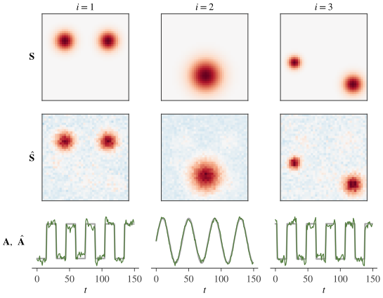
The following script builds a small synthetic data set with three maps on a $40 \times 40$ grid of voxels. Two components have block-design time courses that overlap in time, the third a slow oscillation. After adding Gaussian noise, it runs spatial ICA with symmetric FastICA (Chapter 8第 8 章).

下面的脚本构造一个小型合成数据集：$40 \times 40$ 体素网格上的三张空间图，其中两个成分的时间过程是在时间上相互交叠的组块设计，第三个是缓慢的振荡。加入高斯噪声后，用对称 FastICA（Chapter 8第 8 章）做空间 ICA。

import numpy as np

rng = np.random.default_rng(0)
side, T, n = 40, 150, 3
yy, xx = np.mgrid[0:side, 0:side]
def blob(cy, cx, r):                                  # Gaussian blob on the grid
    return np.exp(-((yy - cy)**2 + (xx - cx)**2) / (2 * r**2)).ravel()
S = np.vstack([blob(12, 10, 3) + blob(12, 30, 3),     # three spatial maps, n x V
               blob(28, 20, 5),
               blob(22, 6, 2) + blob(32, 33, 3)])
t = np.arange(T)
block = ((t // 15) % 2).astype(float)                 # 15 scans on, 15 off
A = np.column_stack([block, np.sin(2 * np.pi * t / 40), np.roll(block, 3)])
X = A @ S + 0.3 * rng.standard_normal((T, side * side))   # T x V data

# Spatial ICA: voxels are the samples. Center each row, PCA-whiten to n dims.
Xc = X - X.mean(axis=1, keepdims=True)
d, E = np.linalg.eigh(Xc @ Xc.T / Xc.shape[1])
d, E = d[-n:], E[:, -n:]
Z = np.diag(d ** -0.5) @ E.T @ Xc                     # n x V, identity covariance

U = np.linalg.qr(rng.standard_normal((n, n)))[0]      # symmetric FastICA, g = tanh
for _ in range(100):
    Y = U @ Z
    U = np.tanh(Y) @ Z.T / Z.shape[1] - np.diag((1 - np.tanh(Y)**2).mean(1)) @ U
    u, _, vt = np.linalg.svd(U)
    U = u @ vt                                        # U <- (U U^T)^(-1/2) U
S_hat = U @ Z                                         # estimated maps
A_hat = E @ np.diag(d ** 0.5) @ U.T                   # estimated time courses

print(np.round(np.corrcoef(A.T)[0, 2], 2))            # true time courses 1 and 3
print(np.round(np.abs(np.corrcoef(S_hat, S)[:n, n:]), 2))
print(np.round(np.abs(np.corrcoef(A_hat.T, A.T)[:n, n:]), 2))

The first line of output is $0.6$, the correlation between the two block-design time courses. The next two print absolute correlations between estimated components (rows) and true components (columns): the maps are recovered with correlations $0.98$, $0.94$ and $0.94$ and the time courses with $0.99$, $0.98$ and $0.99$, in the order $(2, 1, 3)$, an arbitrary permutation as always (Section 1.3第 1.3 节). The off-diagonal time-course correlations of up to $0.55$ only reflect the correlation of the true time courses. Correlated time courses do not prevent spatial ICA from separating the components, because the model places no constraint on $\bA$. Figure 14.1图 14.1 shows the result.

输出的第一行是 $0.6$，即两条组块设计时间过程之间的相关系数。接下来两部分输出估计成分（行）与真实成分（列）之间相关系数的绝对值：空间图的恢复相关系数为 $0.98$、$0.94$、$0.94$，时间过程为 $0.99$、$0.98$、$0.99$，顺序为 $(2, 1, 3)$，同往常一样是一个任意的置换（Section 1.3第 1.3 节）。时间过程之间高达 $0.55$ 的非对角相关，只是反映了真实时间过程之间的相关。时间过程相关并不妨碍空间 ICA 分离各成分，因为这个模型对 $\bA$ 没有任何约束。结果见Figure 14.1图 14.1。

14.3 Spatial versus temporal ICA空间 ICA 与时间 ICA

The same matrix can be factorized with independence imposed on the other factor. Temporal ICA treats the time points as samples and the voxels as sensors. It transposes the model to $\bX^\top = \bS^\top\bA^\top$ and asks the time courses, the columns of $\bA$, to be independent, leaving the maps unconstrained. Both are legitimate models of the same data; they differ in what is assumed to be independent, and they generally give different decompositions. Calhoun, Adalı, Pearlson and Pekar (2001) compared them on fMRI data containing a pair of task-related waveforms and showed that the two can lead to different results, depending on whether the underlying sources are independent in space or in time.

同一个矩阵也可以在另一个因子上施加独立性来分解。时间 ICA 把时间点当作样本、把体素当作传感器：它把模型转置为 $\bX^\top = \bS^\top\bA^\top$，要求时间过程（$\bA$ 的各列）相互独立，而对空间图不加约束。两者都是同一数据的合理模型，区别在于假设哪个因子独立，一般会给出不同的分解。Calhoun、Adalı、Pearlson 与 Pekar（2001）在含有一对任务相关波形的 fMRI 数据上比较了二者，表明根据潜在的源是在空间上独立还是在时间上独立，两种方法可能得出不同的结果。

The singular value decomposition makes the difference precise. Let $\bX$ be centered over voxels and over time, and let $\mathbf{E}_n\bSigma_n\bH_n^\top$ be its truncated SVD with $n$ terms, with orthonormal columns in $\mathbf{E}_n \in \R^{T\times n}$ and $\bH_n \in \R^{V\times n}$; the left singular vectors are the eigenvectors $\mathbf{E}_n$ above, and $\bLambda_n = \bSigma_n^2/V$. Substituting into (14.2), and repeating the computation with the roles of time and space exchanged (Exercise 14.3习题 14.3), gives

奇异值分解能把这一区别说清楚。设 $\bX$ 在体素方向和时间方向都已中心化，$\mathbf{E}_n\bSigma_n\bH_n^\top$ 是它保留 $n$ 项的截断 SVD，$\mathbf{E}_n \in \R^{T\times n}$ 与 $\bH_n \in \R^{V\times n}$ 的列都是单位正交的；左奇异向量就是上文的特征向量 $\mathbf{E}_n$，且 $\bLambda_n = \bSigma_n^2/V$。代入 (14.2)，再把时间与空间的角色互换重复同样的计算（Exercise 14.3习题 14.3），得到

for spatial ICA (first line) and temporal ICA (second line), with orthogonal matrices $\bU$ and $\bU'$ chosen by the respective ICA steps. Both are rotations within the same pair of $n$-dimensional singular subspaces, and both reproduce the same rank-$n$ approximation $\mathbf{E}_n\bSigma_n\bH_n^\top$. They differ in where the singular values go. Spatial ICA makes the maps uncorrelated with unit variance and lets the time courses be correlated; temporal ICA makes the time courses uncorrelated and lets the maps be correlated, that is, overlap. Components whose time courses are correlated, like those of the example above, can be recovered exactly only by spatial ICA; components with overlapping maps but independent time courses only by temporal ICA.

第一行对应空间 ICA，第二行对应时间 ICA，其中正交矩阵 $\bU$ 与 $\bU'$ 由各自的 ICA 步骤选取。两者都是在同一对 $n$ 维奇异子空间内的旋转，也都重现同一个秩 $n$ 近似 $\mathbf{E}_n\bSigma_n\bH_n^\top$。区别在于奇异值放在哪里。空间 ICA 让各张图互不相关且方差为一，而允许时间过程相关；时间 ICA 让时间过程互不相关，而允许空间图相关，也就是相互重叠。时间过程相关的成分（如上例）只有空间 ICA 能准确恢复；空间图重叠而时间过程独立的成分只有时间 ICA 能准确恢复。

In practice spatial ICA dominates fMRI analysis, for three reasons. The first is sample size: spatial ICA estimates an $n\times n$ rotation from $V$ samples, tens of thousands or more, while temporal ICA has only $T$ samples, a few hundred in a typical session. The second is the shape of the sources: the maps of brain networks are sparse, near zero in most voxels and large in a few, which makes them strongly super-Gaussian, matching the source model built into Infomax with the logistic nonlinearity, the algorithm used by McKeown et al. (1998) (Chapter 7第 7 章). The third is that the time courses of different networks are often correlated, through a shared task or shared physiology, which violates temporal independence but does not affect spatial ICA. Temporal ICA becomes feasible with the much higher temporal sampling of accelerated acquisitions; Smith et al. (2012) used it to find temporally independent functional modes whose maps overlap, including several that split the default-mode network into distinct subnetworks.

实践中空间 ICA 在 fMRI 分析中占主导地位，原因有三。其一是样本量：空间 ICA 用 $V$ 个样本（数万甚至更多）估计一个 $n\times n$ 的旋转，而时间 ICA 只有 $T$ 个样本，一次典型扫描不过几百个。其二是源的形态：脑网络的空间图是稀疏的，大多数体素接近零，少数体素取值很大，因而是强超高斯的，这正好符合 McKeown 等（1998）所用的 logistic 非线性 Infomax 内置的源模型（Chapter 7第 7 章）。其三，不同网络的时间过程往往相关，原因可能是共同的任务，也可能是共同的生理过程；这违背了时间独立性，却不影响空间 ICA。加速采集带来更高的时间采样率之后，时间 ICA 变得可行：Smith 等（2012）用它找到了空间图相互重叠的时间独立功能模式，其中有几个把默认模式网络分成了不同的子网络。

14.4 Dimension reduction and model order降维与模型阶数

The number $n$ of components must be chosen before the rotation is estimated, and it shapes the result more than the choice of algorithm. PCA reduction keeps the $n$ leading eigenvectors of $\frac1V\bX\bX^\top$ and discards the rest as noise. If $n$ is too small, distinct networks are merged into one component; if it is too large, networks are split across several components and noise is fitted (Section 11.4第 11.4 节).

成分个数 $n$ 必须在估计旋转之前选定，它对结果的影响比算法的选择更大。PCA 降维保留 $\frac1V\bX\bX^\top$ 的前 $n$ 个特征向量，其余部分作为噪声舍弃。$n$ 太小，不同的网络会被并入同一个成分；$n$ 太大，网络会被拆到几个成分中，噪声也会被拟合进来（Section 11.4第 11.4 节）。

Information criteria such as AIC and MDL estimate $n$ from the eigenvalue spectrum under the assumption of independent samples (Section 11.3第 11.3 节). In fMRI the samples are voxels, which are strongly dependent, not least because of spatial smoothing, and the criteria then overestimate the order. Li, Adalı and Calhoun (2007) subsample the voxel grid to obtain approximately independent samples before applying them. Beckmann and Smith (2004) choose the order that maximizes a Laplace approximation to the Bayesian evidence of probabilistic PCA (Minka, 2000), after adjusting the eigenspectrum for the limited number of samples.

AIC、MDL 等信息准则在样本独立的假设下，根据特征值谱估计 $n$（Section 11.3第 11.3 节）。在 fMRI 中样本是体素，而体素之间依赖很强（空间平滑更加剧了这一点），这些准则因此会高估阶数。Li、Adalı 与 Calhoun（2007）先对体素网格做子采样，得到近似独立的样本，再应用信息准则。Beckmann 与 Smith（2004）则先针对样本数有限对特征值谱作校正，再选择使概率 PCA 的贝叶斯证据的 Laplace 近似（Minka, 2000）最大的阶数。

Such estimates are a guide rather than an answer. On resting-state data, low orders of a few tens give large-scale networks, and higher orders split many of them into smaller subnetworks (Abou-Elseoud et al., 2010). Neither is wrong: the order sets the spatial scale of the decomposition, and studies choose it for the question at hand. Group analyses also reduce each subject's data before the group-level reduction (Chapter 15第 15 章).

这类估计只是参考，而不是答案。在静息态数据上，几十的低阶数给出大尺度网络，更高的阶数则把其中许多网络拆分成更小的子网络（Abou-Elseoud et al., 2010）。两者都不算错：阶数决定了分解的空间尺度，研究者应根据所要回答的问题来选择。组分析还会先对每个被试的数据降维，再做组水平的降维（Chapter 15第 15 章）。

14.5 Algorithms in practice实践中的算法

Any ICA algorithm can rotate the whitened data $\bZ$. Three are common in fMRI.

任何 ICA 算法都可以用来旋转白化后的数据 $\bZ$。fMRI 中常用的有三种。

• Infomax. McKeown et al. (1998) used Infomax (Bell & Sejnowski, 1995) with the logistic nonlinearity, whose implicit source model is super-Gaussian. This suits sparse maps, and Infomax remains a common choice, for example in analyses with the GIFT toolbox. Its fixed nonlinearity is also its weakness: sources that are not super-Gaussian can violate its stability condition (Theorem 7.2定理 7.2), a point that returns in Section 14.7第 14.7 节.
• FastICA. The fixed-point algorithm (Hyvärinen, 1999) with the $\tanh$ or Gaussian nonlinearity is equally widespread and is used in the example above.
• Probabilistic ICA. PICA (Beckmann & Smith, 2004), implemented in the MELODIC tool of the FSL software, models the time series of voxel $v$ as $\bA\bs_v + \bmu + \boldsymbol\eta_v$, where $\bs_v$ collects the $n$ source values at $v$, there are fewer sources than time points, and the Gaussian noise $\boldsymbol\eta_v$ may have a different covariance at each voxel. It estimates the signal subspace and the model order with probabilistic PCA, the rotation with a fixed-point algorithm, and converts the maps into statistics for thresholding (Section 14.6第 14.6 节).

• Infomax。McKeown 等（1998）使用的是带 logistic 非线性函数的 Infomax（Bell & Sejnowski, 1995），其隐含的源模型是超高斯的。这与稀疏的空间图相吻合，Infomax 至今仍是常用的选择，例如在使用 GIFT 工具箱的分析中。固定的非线性函数也是它的弱点：非超高斯的源可能违背它的稳定性条件（Theorem 7.2定理 7.2），Section 14.7第 14.7 节还会回到这一点。
• FastICA。采用 $\tanh$ 或高斯型非线性函数的不动点算法（Hyvärinen, 1999）同样应用广泛，上面的例子用的就是它。
• 概率 ICA。PICA（Beckmann & Smith, 2004）在 FSL 软件的 MELODIC 工具中实现。它把体素 $v$ 的时间序列建模为 $\bA\bs_v + \bmu + \boldsymbol\eta_v$，其中 $\bs_v$ 汇集了 $n$ 个源在 $v$ 处的取值，源的个数少于时间点数，高斯噪声 $\boldsymbol\eta_v$ 的协方差可以随体素而不同。它用概率 PCA 估计信号子空间与模型阶数，用不动点算法估计旋转，并把空间图转换为可用于阈值化的统计量（Section 14.6第 14.6 节）。

Whatever the algorithm, the estimate depends on the random initialization, because ICA contrasts have local optima and their finite-sample landscape is noisy. ICASSO (Himberg, Hyvärinen & Esposito, 2004) runs the algorithm many times, with different initializations or on bootstrap resamples, clusters the estimated components, and reports the most central estimate of each cluster together with a stability index (Section 11.5第 11.5 节); the GIFT toolbox includes it. A high index means that an estimate is reproducible under these perturbations, not that it is correct.

无论用哪种算法，估计结果都依赖于随机初始化，因为 ICA 对比函数存在局部最优，而且有限样本下的目标函数地形带有噪声。ICASSO（Himberg, Hyvärinen & Esposito, 2004）用不同的初始值或在自助重抽样的数据上多次运行算法，对估计出的成分做聚类，报告每一类中最居中的估计以及一个稳定性指标（Section 11.5第 11.5 节）；GIFT 工具箱包含了这一方法。指标高说明估计在这些扰动下可以复现，并不说明它是正确的。

14.6 Reading the components解读成分

Each component $\ba_i\bs_i^\top$ is determined only up to a factor that can move between time course and map, since $\ba_i\bs_i^\top = (c\,\ba_i)(\bs_i/c)^\top$ for every $c \neq 0$ (Section 1.3第 1.3 节). Two conventions make maps comparable. Each map is scaled to z-scores over voxels, dividing it by its standard deviation (the maps of spatial ICA already have mean zero), and the time course is multiplied by the same standard deviation so that the product is unchanged. Map and time course are then flipped together, if necessary, so that the map has positive skewness: its heavy tail of strongly involved voxels points upward. PICA instead divides each map by the voxelwise standard deviation of the residual noise, aiming at a statistic with the same null distribution at every voxel.

每个成分 $\ba_i\bs_i^\top$ 只确定到一个可以在时间过程与空间图之间转移的因子，因为对任意 $c \neq 0$ 都有 $\ba_i\bs_i^\top = (c\,\ba_i)(\bs_i/c)^\top$（Section 1.3第 1.3 节）。有两条约定使空间图可以相互比较。把每张图除以它在体素上的标准差，换算为 z 分数（空间 ICA 的图本来就是零均值的），同时把时间过程乘以同一个标准差，使乘积保持不变。然后在必要时把图和时间过程一起变号，使图的偏度为正，即强烈参与的体素构成的重尾朝上。PICA 则把每张图除以残差噪声在各体素上的标准差，目的是得到在每个体素上零假设分布都相同的统计量。

Thresholds such as $|z| > 2$ or $3$ are descriptive conventions rather than tests: a z-scored ICA map is not a test statistic with a known null distribution, and neighboring voxels are strongly dependent. PICA fits a mixture model to the histogram of each statistic map, with one class for background noise and further classes for activation, and labels a voxel active when its posterior probability of belonging to the activation classes exceeds a chosen level such as 0.5 (Beckmann & Smith, 2004). Components are usually ordered by the variance they explain or by spatial correlation with reference templates.

$|z| > 2$ 或 $3$ 之类的阈值只是描述性的约定，而不是检验：z 分数化的 ICA 图并不是零假设分布已知的检验统计量，而且相邻体素之间依赖很强。PICA 对每张统计量图的直方图拟合一个混合模型，其中一类对应背景噪声，其余各类对应激活；当某体素属于激活类的后验概率超过选定的水平（例如 0.5）时，把它标记为激活（Beckmann & Smith, 2004）。成分通常按其解释的方差排序，或按与参考模板的空间相关排序。

Applied to resting-state data, spatial ICA finds a reproducible set of large-scale networks. Beckmann et al. (2005) reported networks resembling known functional systems such as visual and sensorimotor cortex; Damoiseaux et al. (2006) found ten networks consistent across subjects and sessions, covering motor, visual, auditory, executive and memory-related regions and the default-mode network; and Smith et al. (2009) showed that the major networks found by ICA of resting-state data from 36 subjects correspond closely to networks extracted by ICA from thousands of task activation maps in the BrainMap database.

用于静息态数据时，空间 ICA 能找到一组可复现的大尺度网络。Beckmann 等（2005）报告的网络与视觉皮层、感觉运动皮层等已知功能系统相似；Damoiseaux 等（2006）发现了十个在被试之间和扫描之间都一致的网络，涵盖运动、视觉、听觉、执行与记忆相关脑区以及默认模式网络；Smith 等（2009）则表明，对 36 名被试的静息态数据做 ICA 得到的主要网络，与对 BrainMap 数据库中数千张任务激活图做 ICA 得到的网络高度对应。

Not every component is a network. ICA also isolates structured noise, and this is one of its most practical uses: components caused by head motion, often a rim at the edge of the brain; by cerebrospinal fluid in the ventricles; by white matter; by cardiac and respiratory pulsation near large vessels; and by scanner artifacts, often with time courses dominated by high frequencies. Classifying components by eye is laborious, and two automatic classifiers are widely used. ICA-FIX (Salimi-Khorshidi et al., 2014; Griffanti et al., 2014) computes many spatial and temporal features of each component and feeds them to a hierarchical fusion of classifiers trained on hand-labelled data. ICA-AROMA (Pruim et al., 2015) targets head motion with four features: the maximum robust correlation of the time course with time series derived from the realignment parameters, the high-frequency content of the time course, and the fractions of the map that lie at the edge of the brain and in cerebrospinal fluid. It needs no retraining on new data.

并不是每个成分都是网络。ICA 还能把结构化的噪声单独分离出来，这是它最实用的功能之一：头动造成的成分（常表现为脑边缘的一圈）、脑室中脑脊液造成的成分、白质成分、大血管附近心跳与呼吸搏动造成的成分，以及扫描仪伪迹，它们的时间过程常以高频为主。靠肉眼对成分分类很费力，常用的自动分类器有两种。ICA-FIX（Salimi-Khorshidi et al., 2014; Griffanti et al., 2014）计算每个成分的大量空间与时间特征，送入一个在人工标注数据上训练的分层融合分类器。ICA-AROMA（Pruim et al., 2015）针对头动，只用四个特征：时间过程与由重新对齐参数导出的时间序列之间的最大稳健相关，时间过程的高频成分比例，以及空间图位于脑边缘和位于脑脊液中的比例。它不需要针对新数据重新训练。

Once noise components are labelled, they are removed from the data. Split the estimated time courses into signal and noise columns, $\hat\bA = [\hat\bA_{S},\ \hat\bA_{N}]$, and let $\hat\bB = \hat\bA^+\bX$ be the coefficients of the full regression of the data on all time courses, with corresponding blocks $\hat\bB_S$ and $\hat\bB_N$. The two usual cleanups are

噪声成分一旦标注出来，就要从数据中去除。把估计的时间过程分为信号列和噪声列，$\hat\bA = [\hat\bA_{S},\ \hat\bA_{N}]$，并令 $\hat\bB = \hat\bA^+\bX$ 为数据对全部时间过程做完整回归的系数，相应地分块为 $\hat\bB_S$ 与 $\hat\bB_N$。常用的两种清理方式是

The first, soft or non-aggressive, cleanup removes only what the full regression attributes to the noise components. The second, aggressive, cleanup removes everything the noise time courses can explain, including the part of the signal components that happens to be correlated with them (Exercise 14.4习题 14.4). FIX performs the soft cleanup by default, with the aggressive one as an option, and ICA-AROMA offers both.

第一种是温和（非激进）清理，只去除完整回归归于噪声成分的部分。第二种是激进清理，去除噪声时间过程所能解释的一切，包括信号成分中恰好与噪声时间过程相关的那一部分（Exercise 14.4习题 14.4）。FIX 默认采用温和清理，激进清理作为选项；ICA-AROMA 两种都提供。

14.7 Is spatial independence the right assumption?空间独立是正确的假设吗？

Brain networks overlap, share nodes and interact, so the maps of real networks are unlikely to be exactly independent. Even the synthetic maps of Section 14.2第 14.2 节 are not: their blobs barely overlap, so where one map is large the others are near zero, and their values at a random voxel are dependent. Spatial ICA nevertheless recovered them. What, then, does ICA select for in fMRI?

脑网络相互重叠、共享节点并且相互作用，所以真实网络的空间图不太可能严格独立。就连Section 14.2第 14.2 节中的合成图也不独立：它们的斑块几乎不重叠，一张图取值大的地方其他图都接近零，所以它们在随机体素处的取值并不独立。可空间 ICA 仍然把它们恢复了出来。那么，ICA 在 fMRI 中究竟偏好什么？

Daubechies et al. (2009) argued that Infomax and FastICA succeed on fMRI because they favour sparse components rather than independent ones. In simulations with box-shaped sources they found cases in which independent sources were not separated while dependent but sparse ones were, and they suggested that methods aimed directly at sparsity would suit fMRI better. Calhoun et al. (2013) replied that the failures came from a mismatch between the algorithms' fixed source models, super-Gaussian for Infomax with the logistic nonlinearity and high-kurtosis for the FastICA nonlinearity used, and simulated sources with near-zero kurtosis and bimodal distributions. Infomax with a sub-Gaussian nonlinearity separated those sources well to moderately well, and entropy bound minimization, an algorithm with a flexible density model, separated them in all cases. They concluded that the algorithms do what they are designed to do, find maximally independent components, and that sparsity is not the main driver of their success.

Daubechies 等（2009）认为，Infomax 与 FastICA 在 fMRI 上之所以成功，是因为它们偏好稀疏的成分，而不是独立的成分。在以方块为源的仿真中，他们发现有的情形下独立的源没有被分开，而不独立但稀疏的源反而被分开了；他们据此建议，直接以稀疏性为目标的方法更适合 fMRI。Calhoun 等（2013）回应说，那些失败源于失配：算法内置的源模型是固定的（logistic 非线性的 Infomax 对应超高斯，所用 FastICA 非线性对应高峭度），而仿真中的源峭度接近零、分布呈双峰。改用亚高斯非线性的 Infomax，就能较好或尚可地分离这些源；而采用具有灵活密度模型的熵界最小化算法，在所有情形下都能把它们分开。他们的结论是：这些算法做的正是设计它们去做的事，即寻找最大程度独立的成分，稀疏性并不是它们成功的主要原因。

The theory of Chapter 7第 7 章 explains the mechanism: a contrast with a fixed nonlinearity has a stable separating point only for sources that satisfy its stability condition (Theorem 7.2定理 7.2). In fMRI the useful sources, sparse maps, are super-Gaussian, which is why fixed super-Gaussian nonlinearities work so well and why sparsity and independence are hard to tell apart in practice. Three lessons follow. Treat spatial independence as a working model rather than a literal truth. Prefer algorithms, or nonlinearities, matched to the sources one expects. And check reliability (Section 11.5第 11.5 节) and agreement with independent knowledge before interpreting a component.

Chapter 7第 7 章的理论解释了其中的机制：采用固定非线性函数的对比函数，只对满足其稳定性条件的源才有稳定的分离点（Theorem 7.2定理 7.2）。在 fMRI 中，有用的源（稀疏的空间图）是超高斯的，这正是固定的超高斯非线性函数效果很好的原因，也是实践中很难把稀疏性与独立性区分开的原因。由此得到三条经验：把空间独立当作一个工作模型，而不是字面上的事实；优先选择与预期的源相匹配的算法或非线性函数；在解读某个成分之前，先检查其可靠性（Section 11.5第 11.5 节）以及与独立先验知识是否吻合。

14.8 Exercises习题

14.9 References参考文献