The ICA BookICA 学习书 Yuda Bi

Part III · Chapter 8第三部分 · 第 8 章

FastICAFastICA 算法

The fixed-point algorithm as an approximate Newton method: one-unit, deflation and symmetric versions, convergence rates, and the choice of nonlinearity.

作为近似牛顿法的不动点算法:单单元、逐次提取与对称版本,收敛速度,以及非线性函数的选择。

8.1 A fixed-point view不动点的视角

The gradient algorithms of Chapter 7第 7 章 need a step size, and near a solution they converge only linearly, at a rate set by the smallest eigenvalue of their linearization. FastICA (Hyvärinen & Oja, 1997; Hyvärinen, 1999) takes another route. It works on whitened data, estimates one direction at a time on the unit sphere, and replaces the gradient step by a fixed-point iteration obtained from Newton's method. The result has no step size, converges quadratically or even cubically, and usually needs fewer than ten iterations. This chapter derives the iteration, proves its convergence in source coordinates, builds the versions that estimate several components, and discusses the choice of nonlinearity.

Chapter 7第 7 章中的梯度算法需要选择步长,而且在解附近只是线性收敛,收敛速度由线性化的最小特征值决定。FastICA(Hyvärinen & Oja, 1997; Hyvärinen, 1999)走的是另一条路:它在白化数据上工作,在单位球面上一次估计一个方向,并用由牛顿法导出的不动点迭代代替梯度步。这样得到的算法没有步长,二次甚至三次收敛,通常不到十次迭代就够了。本章推导这一迭代,在源坐标下证明其收敛性,构造同时估计多个成分的版本,并讨论非线性函数的选择。

The setting is that of Chapter 3第 3 章: the data are whitened, z=Vx=A~s\bz = \bV\bx = \tilde\bA\bs with A~\tilde\bA orthogonal (Proposition 3.4命题 3.4), and the sources have zero mean and unit variance. A one-unit method looks for a unit vector w\bw such that y=w⊤zy = \bw^\top\bz is one of the sources. In source coordinates, q=A~⊤w\bq = \tilde\bA^\top\bw is again a unit vector and y=q⊤sy = \bq^\top\bs; the direction w\bw recovers source ii exactly when q=±ei\bq = \pm\be_i, where ei\be_i is the ii-th standard basis vector.

问题的设定与Chapter 3第 3 章相同:数据已经白化,z=Vx=A~s\bz = \bV\bx = \tilde\bA\bs,其中 A~\tilde\bA 是正交矩阵(Proposition 3.4命题 3.4),源均值为零、方差为一。单单元方法寻找一个单位向量 w\bw,使 y=w⊤zy = \bw^\top\bz 恰好是某一个源。在源坐标下,q=A~⊤w\bq = \tilde\bA^\top\bw 仍是单位向量,且 y=q⊤sy = \bq^\top\bs;方向 w\bw 恢复出源 ii,当且仅当 q=±ei\bq = \pm\be_i,这里 ei\be_i 是第 ii 个标准基向量。

8.2 The one-unit contrast单单元对比函数

FastICA maximizes the negentropy approximation of Hyvärinen (1998), introduced in Section 6.7第 6.7 节,

FastICA 最大化Section 6.7第 6.7 节介绍过的 Hyvärinen(1998)负熵近似

JG(w)=[E G(w⊤z)−E G(ν)]2,∥w∥=1,(8.1)J_G(\bw) = \bigl[\E\,G(\bw^\top\bz) - \E\,G(\nu)\bigr]^2, \qquad \|\bw\| = 1,\tag{8.1}

where ν\nu is a standard Gaussian variable and GG is a smooth function. Because z\bz is white, every y=w⊤zy = \bw^\top\bz with ∥w∥=1\|\bw\| = 1 has unit variance, so JGJ_G compares yy with a Gaussian of the same variance. The algorithm uses the derivative g=G′g = G' and its derivative g′g'. Table 8.1表 8.1 lists the three standard choices. For G(u)=u4/4G(u) = u^4/4, E G(y)−E G(ν)=kurt⁡(y)/4\E\,G(y) - \E\,G(\nu) = \kurt(y)/4, and JGJ_G is the squared kurtosis of Chapter 5第 5 章.

其中 ν\nu 是标准高斯变量,GG 是光滑函数。由于 z\bz 是白的,每个满足 ∥w∥=1\|\bw\| = 1 的 y=w⊤zy = \bw^\top\bz 都是单位方差,所以 JGJ_G 是在把 yy 与同方差的高斯变量作比较。算法用到导数 g=G′g = G' 及其导数 g′g'。Table 8.1表 8.1列出了三种标准选择。对 G(u)=u4/4G(u) = u^4/4,有 E G(y)−E G(ν)=kurt⁡(y)/4\E\,G(y) - \E\,G(\nu) = \kurt(y)/4,此时 JGJ_G 就是Chapter 5第 5 章中的峭度平方。

Table 8.1. Standard contrast functions of FastICA (1≤a≤21 \le a \le 2 is a constant, often a=1a = 1) and the quantity λ=E[s g(s)−g′(s)]\lambda = \E[s\,g(s) - g'(s)] that governs their behaviour, for unit-variance uniform and Laplace sources (computed with a=1a = 1 by numerical quadrature). For a Gaussian source λ=0\lambda = 0 for every gg.表 8.1 FastICA 的标准对比函数(1≤a≤21 \le a \le 2 为常数,常取 a=1a = 1),以及决定其行为的量 λ=E[s g(s)−g′(s)]\lambda = \E[s\,g(s) - g'(s)] 在单位方差均匀源和拉普拉斯源下的取值(取 a=1a = 1,用数值积分计算)。对高斯源,任何 gg 都有 λ=0\lambda = 0。
G(u)G(u)g(u)g(u)g′(u)g'(u)λ\lambda, uniformλ\lambda,均匀λ\lambda, Laplaceλ\lambda,拉普拉斯
1alog⁡cosh⁡(au)\frac1a\log\cosh(au)tanh⁡(au)\tanh(au)a(1−tanh⁡2(au))a\bigl(1 - \tanh^2(au)\bigr)0.1260.126−0.148-0.148
−e−u2/2-e^{-u^2/2}u e−u2/2u\,e^{-u^2/2}(1−u2) e−u2/2(1 - u^2)\,e^{-u^2/2}0.2170.217−0.211-0.211
u4/4u^4/4u3u^33u23u^2−1.2-1.233

The source directions are critical points of E G(w⊤z)\E\,G(\bw^\top\bz) on the sphere, and the sign of λi=E[si g(si)−g′(si)]\lambda_i = \E[s_i\,g(s_i) - g'(s_i)] decides their type.

源方向都是 E G(w⊤z)\E\,G(\bw^\top\bz) 在球面上的临界点,而 λi=E[si g(si)−g′(si)]\lambda_i = \E[s_i\,g(s_i) - g'(s_i)] 的符号决定临界点的类型。

Proposition 8.1 (critical points of the one-unit contrast)命题 8.1(单单元对比函数的临界点)

Let GG be twice continuously differentiable, and let the sources be independent with zero mean, unit variance and finite moments of the orders needed below. On the unit sphere, f(q)=E G(q⊤s)f(\bq) = \E\,G(\bq^\top\bs) has a critical point at every ±ei\pm\be_i. It is a strict local maximum if λi>0\lambda_i > 0 and a strict local minimum if λi<0\lambda_i < 0 (Hyvärinen, 1999).

设 GG 二阶连续可微,各源相互独立、均值为零、方差为一,且下面用到的各阶矩有限。在单位球面上,f(q)=E G(q⊤s)f(\bq) = \E\,G(\bq^\top\bs) 在每个 ±ei\pm\be_i 处取临界点。若 λi>0\lambda_i > 0,它是严格局部极大值点;若 λi<0\lambda_i < 0,它是严格局部极小值点(Hyvärinen, 1999)。

Proof.证明

The Euclidean gradient of ff is E[s g(q⊤s)]\E[\bs\,g(\bq^\top\bs)]. At q=ei\bq = \be_i its jj-th component is E[sj] E[g(si)]=0\E[s_j]\,\E[g(s_i)] = 0 for j≠ij \ne i, so the gradient is parallel to ei\be_i and ei\be_i is a critical point on the sphere (the Lagrange condition). For the second order, take i=1i = 1 and move along the sphere: q=(1−∥δ∥2,δ)\bq = (\sqrt{1 - \|\boldsymbol{\delta}\|^2}, \boldsymbol{\delta}) with δ∈Rn−1\boldsymbol{\delta} \in \R^{n-1} small, so y=s1+hy = s_1 + h with h=(1−∥δ∥2−1) s1+∑j≥2δjsjh = (\sqrt{1 - \|\boldsymbol{\delta}\|^2} - 1)\,s_1 + \sum_{j \ge 2}\delta_js_j. Expanding G(s1+h)=G(s1)+g(s1)h+12g′(s1)h2+o(h2)G(s_1 + h) = G(s_1) + g(s_1)h + \tfrac12 g'(s_1)h^2 + o(h^2) and using independence, zero means and unit variances,

ff 的欧氏梯度为 E[s g(q⊤s)]\E[\bs\,g(\bq^\top\bs)]。在 q=ei\bq = \be_i 处,其第 jj 个分量(j≠ij \ne i)为 E[sj] E[g(si)]=0\E[s_j]\,\E[g(s_i)] = 0,所以梯度平行于 ei\be_i,ei\be_i 是球面上的临界点(即 Lagrange 条件)。再看二阶项:取 i=1i = 1,沿球面移动,q=(1−∥δ∥2,δ)\bq = (\sqrt{1 - \|\boldsymbol{\delta}\|^2}, \boldsymbol{\delta}),其中 δ∈Rn−1\boldsymbol{\delta} \in \R^{n-1} 很小,于是 y=s1+hy = s_1 + h,h=(1−∥δ∥2−1) s1+∑j≥2δjsjh = (\sqrt{1 - \|\boldsymbol{\delta}\|^2} - 1)\,s_1 + \sum_{j \ge 2}\delta_js_j。把 G(s1+h)G(s_1 + h) 展开为 G(s1)+g(s1)h+12g′(s1)h2+o(h2)G(s_1) + g(s_1)h + \tfrac12 g'(s_1)h^2 + o(h^2),并利用独立性、零均值与单位方差,得

f(q)=E G(s1)−12∥δ∥2 E[s1g(s1)]+12∥δ∥2 E[g′(s1)]+o(∥δ∥2)=f(e1)−12λ1∥δ∥2+o(∥δ∥2).f(\bq) = \E\,G(s_1) - \tfrac12\|\boldsymbol{\delta}\|^2\,\E[s_1g(s_1)] + \tfrac12\|\boldsymbol{\delta}\|^2\,\E[g'(s_1)] + o(\|\boldsymbol{\delta}\|^2) = f(\be_1) - \tfrac12\lambda_1\|\boldsymbol{\delta}\|^2 + o(\|\boldsymbol{\delta}\|^2).

The term with E[s1g(s1)]\E[s_1g(s_1)] comes from E[g(s1)h]\E[g(s_1)h], using 1−∥δ∥2−1=−12∥δ∥2+O(∥δ∥4)\sqrt{1 - \|\boldsymbol{\delta}\|^2} - 1 = -\tfrac12\|\boldsymbol{\delta}\|^2 + O(\|\boldsymbol{\delta}\|^4) and E[g(s1)sj]=0\E[g(s_1)s_j] = 0 for j≥2j \ge 2; the term with E[g′(s1)]\E[g'(s_1)] comes from 12E[g′(s1)h2]\tfrac12\E[g'(s_1)h^2], using E[g′(s1)(∑jδjsj)2]=E[g′(s1)] ∥δ∥2\E[g'(s_1)(\sum_j\delta_js_j)^2] = \E[g'(s_1)]\,\|\boldsymbol{\delta}\|^2, all other terms being of higher order. The quadratic form −12λ1∥δ∥2-\tfrac12\lambda_1\|\boldsymbol{\delta}\|^2 is negative definite if λ1>0\lambda_1 > 0 and positive definite if λ1<0\lambda_1 < 0.

含 E[s1g(s1)]\E[s_1g(s_1)] 的项来自 E[g(s1)h]\E[g(s_1)h],用到 1−∥δ∥2−1=−12∥δ∥2+O(∥δ∥4)\sqrt{1 - \|\boldsymbol{\delta}\|^2} - 1 = -\tfrac12\|\boldsymbol{\delta}\|^2 + O(\|\boldsymbol{\delta}\|^4) 以及对 j≥2j \ge 2 有 E[g(s1)sj]=0\E[g(s_1)s_j] = 0;含 E[g′(s1)]\E[g'(s_1)] 的项来自 12E[g′(s1)h2]\tfrac12\E[g'(s_1)h^2],用到 E[g′(s1)(∑jδjsj)2]=E[g′(s1)] ∥δ∥2\E[g'(s_1)(\sum_j\delta_js_j)^2] = \E[g'(s_1)]\,\|\boldsymbol{\delta}\|^2,其余各项都是更高阶的。当 λ1>0\lambda_1 > 0 时二次型 −12λ1∥δ∥2-\tfrac12\lambda_1\|\boldsymbol{\delta}\|^2 负定,当 λ1<0\lambda_1 < 0 时正定。

For the kurtosis contrast λi=κi\lambda_i = \kappa_i, consistent with Theorem 5.3定理 5.3: E y4\E\,y^4 is locally maximal at super-Gaussian and minimal at sub-Gaussian sources. For log⁡cosh⁡\log\cosh and the Gaussian-shaped GG the signs are reversed for the laws of Table 8.1表 8.1. Squaring in (8.1) removes the need to know the sign in advance: a critical point ei\be_i of ff is a local maximum of JGJ_G when (E G(si)−E G(ν)) λi>0(\E\,G(s_i) - \E\,G(\nu))\,\lambda_i > 0. This is Theorem 1 of Hyvärinen (1999), stated there for even GG. For kurtosis the product equals κi2/4\kappa_i^2/4, positive whenever κi≠0\kappa_i \ne 0; for the other two GG of the table it is positive for the uniform, Laplace and logistic laws (we checked it by quadrature). As the next sections show, the FastICA iteration itself does not care about the sign at all.

对峭度对比函数,λi=κi\lambda_i = \kappa_i,这与Theorem 5.3定理 5.3一致:E y4\E\,y^4 在超高斯源处取局部极大,在亚高斯源处取局部极小。对 log⁡cosh⁡\log\cosh 和高斯形的 GG,Table 8.1表 8.1中的分布符号正好相反。(8.1) 中的平方使我们无须事先知道符号:当 (E G(si)−E G(ν)) λi>0(\E\,G(s_i) - \E\,G(\nu))\,\lambda_i > 0 时,ff 的临界点 ei\be_i 是 JGJ_G 的局部极大值点;这就是 Hyvärinen(1999)的定理 1,原文假设 GG 为偶函数。对峭度,这个乘积等于 κi2/4\kappa_i^2/4,只要 κi≠0\kappa_i \ne 0 就为正;对表中另两种 GG,它在均匀、拉普拉斯和 logistic 分布下都为正(我们用数值积分验证过)。后面几节将表明,FastICA 迭代本身根本不在乎这个符号。

8.3 Derivation as an approximate Newton method作为近似牛顿法的推导

The optima of E G(w⊤z)\E\,G(\bw^\top\bz) under ∥w∥2=1\|\bw\|^2 = 1 satisfy the Lagrange condition

E G(w⊤z)\E\,G(\bw^\top\bz) 在约束 ∥w∥2=1\|\bw\|^2 = 1 下的最优点满足 Lagrange 条件

F(w)=E[z g(w⊤z)]−β w=0,β=E[w⋆⊤z  g(w⋆⊤z)],(8.2)F(\bw) = \E\bigl[\bz\,g(\bw^\top\bz)\bigr] - \beta\,\bw = \bzero, \qquad \beta = \E\bigl[\bw_\star^\top\bz\;g(\bw_\star^\top\bz)\bigr],\tag{8.2}

where w⋆\bw_\star is the optimum and the value of the multiplier β\beta follows by multiplying the condition by w⋆⊤\bw_\star^\top. Newton's method for (8.2) needs the Jacobian E[zz⊤g′(w⊤z)]−βI\E[\bz\bz^\top g'(\bw^\top\bz)] - \beta\bI. Its first term is the expensive part, and the whiteness of z\bz suggests the approximation

其中 w⋆\bw_\star 是最优点,乘子 β\beta 的值可由条件两边左乘 w⋆⊤\bw_\star^\top 得到。对 (8.2) 用牛顿法,需要雅可比矩阵 E[zz⊤g′(w⊤z)]−βI\E[\bz\bz^\top g'(\bw^\top\bz)] - \beta\bI。其中第一项计算代价最大,而 z\bz 是白的这一事实提示我们作近似

E[zz⊤g′(w⊤z)]≈E[zz⊤] E[g′(w⊤z)]=E[g′(w⊤z)] I,\E\bigl[\bz\bz^\top g'(\bw^\top\bz)\bigr] \approx \E\bigl[\bz\bz^\top\bigr]\,\E\bigl[g'(\bw^\top\bz)\bigr] = \E\bigl[g'(\bw^\top\bz)\bigr]\,\bI,

which ignores the dependence between zz⊤\bz\bz^\top and g′(w⊤z)g'(\bw^\top\bz). At a source direction it is nevertheless exact in every direction orthogonal to w\bw and wrong only along w\bw itself, which the normalization takes care of (Exercise 8.5习题 8.5). With a diagonal Jacobian the Newton step is

这一近似忽略了 zz⊤\bz\bz^\top 与 g′(w⊤z)g'(\bw^\top\bz) 之间的相依性。尽管如此,在源方向上,它在与 w\bw 正交的所有方向上都是精确的,只在 w\bw 本身的方向上有误差,而这个方向由归一化处理(Exercise 8.5习题 8.5)。雅可比矩阵变成对角阵后,牛顿步为

w+=w−E[z g(w⊤z)]−βwE[g′(w⊤z)]−β.\bw^+ = \bw - \frac{\E[\bz\,g(\bw^\top\bz)] - \beta\bw}{\E[g'(\bw^\top\bz)] - \beta}.

Multiplying by the scalar β−E[g′(w⊤z)]\beta - \E[g'(\bw^\top\bz)] changes only the length and possibly the sign of w+\bw^+, both of which the subsequent normalization ignores up to sign. The β\beta terms then cancel and we obtain the FastICA update

两边乘以标量 β−E[g′(w⊤z)]\beta - \E[g'(\bw^\top\bz)],只改变 w+\bw^+ 的长度以及可能改变其符号,而随后的归一化在相差符号的意义下忽略这两者。这样 β\beta 项相互抵消,得到 FastICA 的更新规则

w+=E[z g(w⊤z)]−E[g′(w⊤z)] w,w←w+/∥w+∥.(8.3)\bw^+ = \E\bigl[\bz\,g(\bw^\top\bz)\bigr] - \E\bigl[g'(\bw^\top\bz)\bigr]\,\bw, \qquad \bw \leftarrow \bw^+/\|\bw^+\|.\tag{8.3}

There is no step size and no β\beta to estimate. Because a factor of either sign was dropped, w\bw may flip sign from one iteration to the next; convergence is therefore judged by ∣w+⊤w∣→1|\bw^{+\top}\bw| \to 1 for the normalized iterates, not by w+−w→0\bw^+ - \bw \to \bzero.

这里既没有步长,也不需要估计 β\beta。由于丢掉的因子可正可负,w\bw 可能在相邻两次迭代之间改变符号;因此收敛性应当用归一化迭代满足 ∣w+⊤w∣→1|\bw^{+\top}\bw| \to 1 来判断,而不是用 w+−w→0\bw^+ - \bw \to \bzero。

Algorithm 8.2 (one-unit FastICA)算法 8.2(单单元 FastICA)

  1. Center and whiten the data: z(t)=Vx(t)\bz(t) = \bV\bx(t), t=1,…,Tt = 1, \dots, T.
  2. Choose GG from Table 8.1表 8.1 and a random unit vector w\bw.
  3. Compute w+=E^[z g(w⊤z)]−E^[g′(w⊤z)] w\bw^+ = \hat\E[\bz\,g(\bw^\top\bz)] - \hat\E[g'(\bw^\top\bz)]\,\bw, with sample averages E^\hat\E over tt.
  4. Set wnew=w+/∥w+∥\bw_{\text{new}} = \bw^+/\|\bw^+\|.
  5. If 1−∣wnew⊤w∣1 - |\bw_{\text{new}}^\top\bw| is below a tolerance, stop; otherwise set w=wnew\bw = \bw_{\text{new}} and return to step 3.
  6. Output y(t)=w⊤z(t)y(t) = \bw^\top\bz(t), the estimated source, and w⊤V\bw^\top\bV, the corresponding row of the unmixing matrix.
  1. 中心化并白化数据:z(t)=Vx(t)\bz(t) = \bV\bx(t),t=1,…,Tt = 1, \dots, T。
  2. 从Table 8.1表 8.1中选取 GG,并随机取一个单位向量 w\bw。
  3. 计算 w+=E^[z g(w⊤z)]−E^[g′(w⊤z)] w\bw^+ = \hat\E[\bz\,g(\bw^\top\bz)] - \hat\E[g'(\bw^\top\bz)]\,\bw,其中 E^\hat\E 表示对 tt 的样本平均。
  4. 令 wnew=w+/∥w+∥\bw_{\text{new}} = \bw^+/\|\bw^+\|。
  5. 若 1−∣wnew⊤w∣1 - |\bw_{\text{new}}^\top\bw| 小于容差则停止;否则令 w=wnew\bw = \bw_{\text{new}},回到第 3 步。
  6. 输出估计的源 y(t)=w⊤z(t)y(t) = \bw^\top\bz(t),以及解混矩阵中对应的行 w⊤V\bw^\top\bV。

8.4 Convergence收敛性

In source coordinates the population iteration reads q+=E[s g(q⊤s)]−E[g′(q⊤s)] q\bq^+ = \E[\bs\,g(\bq^\top\bs)] - \E[g'(\bq^\top\bs)]\,\bq, followed by normalization, because A~⊤z=s\tilde\bA^\top\bz = \bs and w⊤z=q⊤s\bw^\top\bz = \bq^\top\bs. For the kurtosis nonlinearity g(u)=u3g(u) = u^3 it can be solved in closed form. Expanding (q⊤s)3(\bq^\top\bs)^3, the moment E[sisjsksl]\E[s_is_js_ks_l] of independent, zero-mean, unit-variance sources vanishes unless the indices pair up, so

由于 A~⊤z=s\tilde\bA^\top\bz = \bs 且 w⊤z=q⊤s\bw^\top\bz = \bq^\top\bs,在源坐标下总体迭代为 q+=E[s g(q⊤s)]−E[g′(q⊤s)] q\bq^+ = \E[\bs\,g(\bq^\top\bs)] - \E[g'(\bq^\top\bs)]\,\bq,然后归一化。对峭度非线性 g(u)=u3g(u) = u^3,这一迭代可以显式求解。展开 (q⊤s)3(\bq^\top\bs)^3;对独立、零均值、单位方差的源,矩 E[sisjsksl]\E[s_is_js_ks_l] 只有在下标两两配对时才不为零,所以

E[si(q⊤s)3]=E[si4] qi3+3 qi∑m≠iqm2=(κi+3) qi3+3 qi (1−qi2)=κi qi3+3 qi,\E\bigl[s_i(\bq^\top\bs)^3\bigr] = \E[s_i^4]\,q_i^3 + 3\,q_i\sum_{m \ne i}q_m^2 = (\kappa_i + 3)\,q_i^3 + 3\,q_i\,(1 - q_i^2) = \kappa_i\,q_i^3 + 3\,q_i,

using ∥q∥=1\|\bq\| = 1. Since E[g′(q⊤s)]=3 E[(q⊤s)2]=3\E[g'(\bq^\top\bs)] = 3\,\E[(\bq^\top\bs)^2] = 3, the update is simply qi+=κiqi3q_i^+ = \kappa_iq_i^3: each coordinate is cubed and weighted by the kurtosis of its source. The identity holds exactly, even for skewed sources; we checked it to machine precision with discrete sources whose expectations can be computed exactly.

这里用到了 ∥q∥=1\|\bq\| = 1。由于 E[g′(q⊤s)]=3 E[(q⊤s)2]=3\E[g'(\bq^\top\bs)] = 3\,\E[(\bq^\top\bs)^2] = 3,更新就是简单的 qi+=κiqi3q_i^+ = \kappa_iq_i^3:每个坐标先取立方,再乘以对应源的峭度。这一恒等式精确成立,对有偏度的源也一样;我们用可以精确计算期望的离散源验证过,误差在机器精度以内。

Theorem 8.3 (convergence of one-unit FastICA)定理 8.3(单单元 FastICA 的收敛性)

Let the sources be independent with zero mean and unit variance, and consider the population iteration q+=E[s g(q⊤s)]−E[g′(q⊤s)] q\bq^+ = \E[\bs\,g(\bq^\top\bs)] - \E[g'(\bq^\top\bs)]\,\bq, q←q+/∥q+∥\bq \leftarrow \bq^+/\|\bq^+\|.

设各源相互独立、均值为零、方差为一,考虑总体迭代 q+=E[s g(q⊤s)]−E[g′(q⊤s)] q\bq^+ = \E[\bs\,g(\bq^\top\bs)] - \E[g'(\bq^\top\bs)]\,\bq,q←q+/∥q+∥\bq \leftarrow \bq^+/\|\bq^+\|。

(a) Kurtosis (Hyvärinen & Oja, 1997). For g(u)=u3g(u) = u^3 and sources with finite fourth moments, qi+=κiqi3q_i^+ = \kappa_iq_i^3 for every ii. If the index i⋆i^\star that maximizes ∣κi∣ ∣qi(0)∣\sqrt{|\kappa_i|}\,|q_i^{(0)}| is unique, the iterates converge to ±ei⋆\pm\be_{i^\star} up to sign, and for every j≠i⋆j \ne i^\star the ratios ρj(k)=∣qj(k)/qi⋆(k)∣\rho_j^{(k)} = |q_j^{(k)}/q_{i^\star}^{(k)}| satisfy ρj(k+1)=(∣κj∣/∣κi⋆∣) (ρj(k))3\rho_j^{(k+1)} = (|\kappa_j|/|\kappa_{i^\star}|)\,(\rho_j^{(k)})^3: the convergence is cubic.

(a)峭度(Hyvärinen & Oja, 1997)。对 g(u)=u3g(u) = u^3 且源的四阶矩有限,对每个 ii 都有 qi+=κiqi3q_i^+ = \kappa_iq_i^3。若使 ∣κi∣ ∣qi(0)∣\sqrt{|\kappa_i|}\,|q_i^{(0)}| 最大的下标 i⋆i^\star 唯一,则迭代在相差符号的意义下收敛到 ±ei⋆\pm\be_{i^\star},并且对每个 j≠i⋆j \ne i^\star,比值 ρj(k)=∣qj(k)/qi⋆(k)∣\rho_j^{(k)} = |q_j^{(k)}/q_{i^\star}^{(k)}| 满足 ρj(k+1)=(∣κj∣/∣κi⋆∣) (ρj(k))3\rho_j^{(k+1)} = (|\kappa_j|/|\kappa_{i^\star}|)\,(\rho_j^{(k)})^3:收敛是三次的。

(b) General gg (convergence rates: Hyvärinen, 1999; the constant cijc_{ij} is computed in the proof below). Let gg be three times differentiable with bounded third derivative, let the sources have finite fourth moments, and let λi=E[si g(si)−g′(si)]≠0\lambda_i = \E[s_i\,g(s_i) - g'(s_i)] \ne 0. Then ei\be_i is a fixed point up to sign, and near it the ratios rj=qj/qir_j = q_j/q_i, j≠ij \ne i, satisfy

(b)一般的 gg(收敛阶见 Hyvärinen, 1999;常数 cijc_{ij} 由下面的证明给出)。设 gg 三阶可微且三阶导数有界,源的四阶矩有限,且 λi=E[si g(si)−g′(si)]≠0\lambda_i = \E[s_i\,g(s_i) - g'(s_i)] \ne 0。则 ei\be_i 在相差符号的意义下是不动点,且在其附近,比值 rj=qj/qir_j = q_j/q_i(j≠ij \ne i)满足

rj+=cij rj2+O(∥r∥3),cij=E[g′′(si)]  E[sj3]2 λi.(8.4)r_j^+ = c_{ij}\,r_j^2 + O(\|\mathbf{r}\|^3), \qquad c_{ij} = \frac{\E[g''(s_i)]\;\E[s_j^3]}{2\,\lambda_i}.\tag{8.4}

The convergence is therefore at least quadratic, and cubic if E[g′′(si)] E[sj3]=0\E[g''(s_i)]\,\E[s_j^3] = 0 for all j≠ij \ne i, for example when gg is odd and sis_i is symmetric, or when all other sources are symmetric.

因此收敛至少是二次的;若对所有 j≠ij \ne i 都有 E[g′′(si)] E[sj3]=0\E[g''(s_i)]\,\E[s_j^3] = 0,则是三次的,例如 gg 为奇函数且 sis_i 对称,或者其余各源都对称。

Proof.证明

(a) The identity was derived above. Put ui=∣κi∣ qiu_i = \sqrt{|\kappa_i|}\,q_i. The unnormalized update gives ∣κi∣ qi+=sign⁡(κi) ui3\sqrt{|\kappa_i|}\,q_i^+ = \sign(\kappa_i)\,u_i^3, and normalization multiplies all coordinates by the same positive number, so ∣uj(k)/ui⋆(k)∣=∣uj(0)/ui⋆(0)∣3k|u_j^{(k)}/u_{i^\star}^{(k)}| = |u_j^{(0)}/u_{i^\star}^{(0)}|^{3^k}. By uniqueness of i⋆i^\star the base is below 1 (coordinates with κj=0\kappa_j = 0 vanish after one step), hence all ratios tend to zero and q(k)\bq^{(k)} approaches ±ei⋆\pm\be_{i^\star}; in particular κi⋆≠0\kappa_{i^\star} \ne 0 and qi⋆(0)≠0q_{i^\star}^{(0)} \ne 0, so q+\bq^+ never vanishes. The recursion for ρj\rho_j is ∣κjqj3∣/∣κi⋆qi⋆3∣|\kappa_jq_j^3|/|\kappa_{i^\star}q_{i^\star}^3|.

(a)恒等式已在上文推出。令 ui=∣κi∣ qiu_i = \sqrt{|\kappa_i|}\,q_i。未归一化的更新给出 ∣κi∣ qi+=sign⁡(κi) ui3\sqrt{|\kappa_i|}\,q_i^+ = \sign(\kappa_i)\,u_i^3,而归一化把所有坐标乘以同一个正数,所以 ∣uj(k)/ui⋆(k)∣=∣uj(0)/ui⋆(0)∣3k|u_j^{(k)}/u_{i^\star}^{(k)}| = |u_j^{(0)}/u_{i^\star}^{(0)}|^{3^k}。由 i⋆i^\star 的唯一性,底数小于 1(κj=0\kappa_j = 0 的坐标在一步之后就变为零),所以所有比值都趋于零,q(k)\bq^{(k)} 趋于 ±ei⋆\pm\be_{i^\star};特别地 κi⋆≠0\kappa_{i^\star} \ne 0 且 qi⋆(0)≠0q_{i^\star}^{(0)} \ne 0,因此 q+\bq^+ 永不为零。ρj\rho_j 的递推就是 ∣κjqj3∣/∣κi⋆qi⋆3∣|\kappa_jq_j^3|/|\kappa_{i^\star}q_{i^\star}^3|。

(b) At q=ei\bq = \be_i the update is E[s g(si)]−E[g′(si)] ei=λiei\E[\bs\,g(s_i)] - \E[g'(s_i)]\,\be_i = \lambda_i\be_i, because E[sjg(si)]=0\E[s_jg(s_i)] = 0 for j≠ij \ne i; so ei\be_i is fixed up to the sign of λi\lambda_i. Near it write q=qiei+δ\bq = q_i\be_i + \boldsymbol{\delta} with δ⊥ei\boldsymbol{\delta} \perp \be_i and qi=1−∥δ∥2q_i = \sqrt{1 - \|\boldsymbol{\delta}\|^2}, and y=si+hy = s_i + h with h=(qi−1)si+∑k≠iδkskh = (q_i - 1)s_i + \sum_{k \ne i}\delta_ks_k. Taylor's theorem with the bounded third derivative gives, for j≠ij \ne i,

(b)在 q=ei\bq = \be_i 处,由于对 j≠ij \ne i 有 E[sjg(si)]=0\E[s_jg(s_i)] = 0,更新为 E[s g(si)]−E[g′(si)] ei=λiei\E[\bs\,g(s_i)] - \E[g'(s_i)]\,\be_i = \lambda_i\be_i;所以 ei\be_i 在相差 λi\lambda_i 的符号的意义下不动。在其附近记 q=qiei+δ\bq = q_i\be_i + \boldsymbol{\delta},其中 δ⊥ei\boldsymbol{\delta} \perp \be_i,qi=1−∥δ∥2q_i = \sqrt{1 - \|\boldsymbol{\delta}\|^2},并记 y=si+hy = s_i + h,h=(qi−1)si+∑k≠iδkskh = (q_i - 1)s_i + \sum_{k \ne i}\delta_ks_k。由三阶导数有界的 Taylor 定理,对 j≠ij \ne i,

E[sj g(y)]=E[sjg(si)]⏟0+E[sj g′(si) h]⏟δjE[g′(si)]+12E[sj g′′(si) h2]⏟E[g′′(si)] E[sj3] δj2+O(∥δ∥3)+O(∥δ∥3),\E[s_j\,g(y)] = \underbrace{\E[s_jg(s_i)]}_{0} + \underbrace{\E[s_j\,g'(s_i)\,h]}_{\delta_j\E[g'(s_i)]} + \tfrac12\underbrace{\E[s_j\,g''(s_i)\,h^2]}_{\E[g''(s_i)]\,\E[s_j^3]\,\delta_j^2 + O(\|\boldsymbol{\delta}\|^3)} + O(\|\boldsymbol{\delta}\|^3),

where independence and zero means kill every other term (the factor qi−1q_i - 1 is of order ∥δ∥2\|\boldsymbol{\delta}\|^2). Similarly E[g′(y)]=E[g′(si)]+O(∥δ∥2)\E[g'(y)] = \E[g'(s_i)] + O(\|\boldsymbol{\delta}\|^2), because E[g′′(si)h]=(qi−1)E[sig′′(si)]\E[g''(s_i)h] = (q_i - 1)\E[s_ig''(s_i)]. The jj-th coordinate of the unnormalized update is therefore uj=E[sjg(y)]−E[g′(y)] δj=12E[g′′(si)]E[sj3] δj2+O(∥δ∥3)u_j = \E[s_jg(y)] - \E[g'(y)]\,\delta_j = \tfrac12\E[g''(s_i)]\E[s_j^3]\,\delta_j^2 + O(\|\boldsymbol{\delta}\|^3): the first-order terms cancel. The ii-th coordinate is ui=λi+O(∥δ∥)u_i = \lambda_i + O(\|\boldsymbol{\delta}\|). Normalization does not change ratios, so rj+=uj/uir_j^+ = u_j/u_i, and since δj=rj (1+O(∥r∥2))\delta_j = r_j\,(1 + O(\|\mathbf{r}\|^2)), (8.4) follows.

其中独立性和零均值使其余各项全部为零(因子 qi−1q_i - 1 是 ∥δ∥2\|\boldsymbol{\delta}\|^2 阶的)。类似地,由于 E[g′′(si)h]=(qi−1)E[sig′′(si)]\E[g''(s_i)h] = (q_i - 1)\E[s_ig''(s_i)],有 E[g′(y)]=E[g′(si)]+O(∥δ∥2)\E[g'(y)] = \E[g'(s_i)] + O(\|\boldsymbol{\delta}\|^2)。因此未归一化更新的第 jj 个坐标为 uj=E[sjg(y)]−E[g′(y)] δj=12E[g′′(si)]E[sj3] δj2+O(∥δ∥3)u_j = \E[s_jg(y)] - \E[g'(y)]\,\delta_j = \tfrac12\E[g''(s_i)]\E[s_j^3]\,\delta_j^2 + O(\|\boldsymbol{\delta}\|^3):一阶项相互抵消。第 ii 个坐标为 ui=λi+O(∥δ∥)u_i = \lambda_i + O(\|\boldsymbol{\delta}\|)。归一化不改变比值,所以 rj+=uj/uir_j^+ = u_j/u_i;再由 δj=rj (1+O(∥r∥2))\delta_j = r_j\,(1 + O(\|\mathbf{r}\|^2)) 即得 (8.4)。

Three consequences are worth stating. First, the iteration converges to source directions whether they are maxima or minima of E G\E\,G: only λi≠0\lambda_i \ne 0 matters, so FastICA finds sub- and super-Gaussian sources with the same nonlinearity. When λi<0\lambda_i < 0 the vector flips sign at every step, which is why convergence is tested through ∣w+⊤w∣|\bw^{+\top}\bw|. Second, part (a) is a global statement: for a random start, ties in ∣κi∣ ∣qi(0)∣\sqrt{|\kappa_i|}\,|q_i^{(0)}| have probability zero, so the kurtosis iteration converges from almost every starting point. Part (b) is local. Third, a Gaussian source has λi=0\lambda_i = 0 (Stein's lemma) and is never a fixed point; with kurtosis its coordinate is set to zero in one step (Exercise 8.2习题 8.2).

有三点推论值得一提。第一,无论源方向是 E G\E\,G 的极大值点还是极小值点,迭代都会收敛到它:要紧的只是 λi≠0\lambda_i \ne 0,所以 FastICA 用同一个非线性函数就能找到亚高斯源和超高斯源。当 λi<0\lambda_i < 0 时,向量每一步都改变符号,这就是要用 ∣w+⊤w∣|\bw^{+\top}\bw| 来检验收敛的原因。第二,(a)是全局性的结论:随机初始化时,∣κi∣ ∣qi(0)∣\sqrt{|\kappa_i|}\,|q_i^{(0)}| 出现并列的概率为零,所以峭度迭代几乎从任何起点出发都收敛。(b)则是局部结论。第三,高斯源满足 λi=0\lambda_i = 0(Stein 引理),永远不是不动点;用峭度时,它对应的坐标一步之内就被置为零(Exercise 8.2习题 8.2)。

Example 8.4 (the kurtosis iteration in two dimensions)例 8.4(二维情形下的峭度迭代)

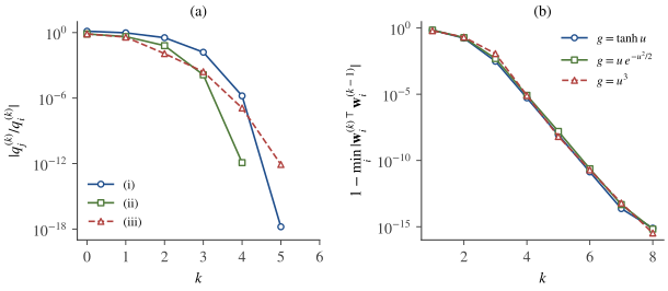
Take a uniform source (κ1=−1.2\kappa_1 = -1.2) and a Laplace source (κ2=3\kappa_2 = 3), and start from q(0)=(0.8,0.6)\bq^{(0)} = (0.8, 0.6), which is closer to the first source. Since 1.2×0.8≈0.876<3×0.6≈1.039\sqrt{1.2} \times 0.8 \approx 0.876 < \sqrt{3} \times 0.6 \approx 1.039, part (a) predicts convergence to the second source, with ρ(k+1)=0.4 (ρ(k))3\rho^{(k+1)} = 0.4\,(\rho^{(k)})^3 for ρ=∣q1/q2∣\rho = |q_1/q_2|. The iterates are q(1)=(−0.688,0.726)\bq^{(1)} = (-0.688, 0.726), q(2)=(0.323,0.946)\bq^{(2)} = (0.323, 0.946), q(3)=(−0.0159,0.99987)\bq^{(3)} = (-0.0159, 0.99987) and q(4)=(1.6×10−6,1.0)\bq^{(4)} = (1.6 \times 10^{-6}, 1.0), and ρ\rho runs through 1.33, 0.948, 0.341, 0.0159, 1.6×10⁻⁶, 1.6×10−181.33,\ 0.948,\ 0.341,\ 0.0159,\ 1.6 \times 10^{-6},\ 1.6 \times 10^{-18}. The number of correct digits roughly triples at each step once the iterate is close, and the first coordinate alternates in sign because κ1<0\kappa_1 < 0.

取一个均匀源(κ1=−1.2\kappa_1 = -1.2)和一个拉普拉斯源(κ2=3\kappa_2 = 3),从更靠近第一个源的 q(0)=(0.8,0.6)\bq^{(0)} = (0.8, 0.6) 出发。由于 1.2×0.8≈0.876<3×0.6≈1.039\sqrt{1.2} \times 0.8 \approx 0.876 < \sqrt{3} \times 0.6 \approx 1.039,(a)预言迭代收敛到第二个源,且 ρ=∣q1/q2∣\rho = |q_1/q_2| 满足 ρ(k+1)=0.4 (ρ(k))3\rho^{(k+1)} = 0.4\,(\rho^{(k)})^3。迭代依次为 q(1)=(−0.688,0.726)\bq^{(1)} = (-0.688, 0.726),q(2)=(0.323,0.946)\bq^{(2)} = (0.323, 0.946),q(3)=(−0.0159,0.99987)\bq^{(3)} = (-0.0159, 0.99987),q(4)=(1.6×10−6,1.0)\bq^{(4)} = (1.6 \times 10^{-6}, 1.0),而 ρ\rho 依次取 1.33, 0.948, 0.341, 0.0159, 1.6×10⁻⁶, 1.6×10−181.33,\ 0.948,\ 0.341,\ 0.0159,\ 1.6 \times 10^{-6},\ 1.6 \times 10^{-18}。一旦迭代足够接近,正确数字的位数大约每步变为三倍;由于 κ1<0\kappa_1 < 0,第一个坐标的符号交替变化。

Two log-scale plots. Left: error ratios of three population FastICA iterations against the iteration number; the kurtosis example and the tanh iteration with symmetric sources fall super-exponentially to below 1e-12 within four or five steps, the tanh iteration with skewed sources more slowly. Right: the convergence measure of symmetric FastICA on data for three nonlinearities, all falling from about 1 to about 1e-15 in eight iterations.
Figure 8.1. (a) Population iterations with exact expectations: (i) the kurtosis example above; (ii) g=tanh⁡g = \tanh with a uniform and a Laplace source, cubic since the sources are symmetric; (iii) g=tanh⁡g = \tanh with two centered exponential sources, quadratic, with ∣r(k+1)∣/(r(k))2→1.806=∣c12∣|r^{(k+1)}|/(r^{(k)})^2 \to 1.806 = |c_{12}|, where c12=−1.806c_{12} = -1.806 is the constant of (8.4). (b) Symmetric FastICA on the four-source example of Section 8.5第 8.5 节 (T=10000T = 10000) with three nonlinearities; the curves show 1−min⁡i∣wi(k)⊤wi(k−1)∣1 - \min_i|\bw_i^{(k)\top}\bw_i^{(k-1)}|.图 8.1 (a)用精确期望计算的总体迭代:(i)上面的峭度例子;(ii)g=tanh⁡g = \tanh,一个均匀源和一个拉普拉斯源,由于源对称而三次收敛;(iii)g=tanh⁡g = \tanh,两个中心化的指数分布源,二次收敛,且 ∣r(k+1)∣/(r(k))2→1.806=∣c12∣|r^{(k+1)}|/(r^{(k)})^2 \to 1.806 = |c_{12}|,其中 c12=−1.806c_{12} = -1.806 是 (8.4) 中的常数。(b)在Section 8.5第 8.5 节的四源例子(T=10000T = 10000)上用三种非线性函数运行对称 FastICA;曲线为 1−min⁡i∣wi(k)⊤wi(k−1)∣1 - \min_i|\bw_i^{(k)\top}\bw_i^{(k-1)}|。

With a finite sample the iteration uses E^\hat\E and converges to a fixed point of the sample map, which lies within O(T−1/2)O(T^{-1/2}) of the population fixed point; its accuracy is the subject of Theorem 10.8定理 10.8. At that point the derivative of the sample map is no longer exactly zero but of the order of the sampling error. In our experiments with g=tanh⁡g = \tanh and TT from 10310^3 to 10610^6 its norm was of the order of 1/T1/\sqrt{T}, typically a few times 1/T1/\sqrt{T}, with a factor that depended on the sources and on the sample. The final iterations therefore converge linearly, but with a ratio so small that this is rarely visible. In the run of Figure 8.1图 8.1(b), with T=104T = 10^4, the measure drops by a factor of about 600 per iteration at the end, so the angle between successive iterates shrinks by a factor of about 25, a contraction of about 4/T4/\sqrt{T}.

在有限样本下,迭代使用 E^\hat\E,收敛到样本映射的不动点,它与总体不动点相距 O(T−1/2)O(T^{-1/2});其精度是Theorem 10.8定理 10.8的主题。在这个点上,样本映射的导数不再恰好为零,而是与抽样误差同阶。在我们用 g=tanh⁡g = \tanh 做的实验中,对 TT 从 10310^3 到 10610^6,该导数的范数都是 1/T1/\sqrt{T} 量级,通常是 1/T1/\sqrt{T} 的几倍,倍数随源和样本而变。因此最后几次迭代是线性收敛的,但收敛比小到几乎看不出来。在Figure 8.1图 8.1(b)的运行中(T=104T = 10^4),最后阶段度量值每次迭代约缩小为原来的 1/600,于是相邻迭代之间的夹角每次约缩小为原来的 1/25,即收缩比约为 4/T4/\sqrt{T}。

8.5 Estimating several components估计多个成分

Running the one-unit algorithm nn times from random starts would often find the same source several times. Since the columns of A~\tilde\bA are orthonormal, the rows wi⊤\bw_i^\top of the orthogonal unmixing matrix U\bU must be orthonormal too, and FastICA enforces this in one of two ways. In this section, as in the FastICA literature, W\bW denotes the matrix with rows wi⊤\bw_i^\top, which acts on whitened data and is the orthogonal matrix U\bU of Table 1.1表 1.1; the unmixing matrix for x\bx is WV\bW\bV.

从随机起点把单单元算法独立运行 nn 次,往往会多次找到同一个源。由于 A~\tilde\bA 的列是标准正交的,正交解混矩阵 U\bU 的各行 wi⊤\bw_i^\top 也必须标准正交,FastICA 用以下两种方式之一来保证这一点。本节沿用 FastICA 文献的习惯,用 W\bW 表示以 wi⊤\bw_i^\top 为行、作用于白化数据的矩阵,即Table 1.1表 1.1中的正交矩阵 U\bU;对 x\bx 的解混矩阵是 WV\bW\bV。

Deflation. Estimate the vectors one after another. While iterating for wp\bw_p, follow each update by a Gram–Schmidt step against the vectors already found, wp←wp−∑j<p(wp⊤wj) wj\bw_p \leftarrow \bw_p - \sum_{j < p}(\bw_p^\top\bw_j)\,\bw_j, and then normalize. If w1,…,wp−1\bw_1, \dots, \bw_{p-1} were exact source directions, the remaining sources would span exactly the orthogonal complement, and the iteration there is again a one-unit problem with fewer sources, so Theorem 8.3定理 8.3 applies. With estimated vectors, however, each error tilts the subspace in which all later vectors must lie, so errors accumulate along the sequence; the last vector has no freedom left at all, being the unit vector orthogonal to the others. The order in which sources come out depends on the starting points and the contrast, not on any property chosen by the user.

逐个提取(紧缩)。依次估计各个向量。在迭代求 wp\bw_p 时,每次更新之后都对已经求得的向量做一次 Gram–Schmidt 正交化,wp←wp−∑j<p(wp⊤wj) wj\bw_p \leftarrow \bw_p - \sum_{j < p}(\bw_p^\top\bw_j)\,\bw_j,然后归一化。如果 w1,…,wp−1\bw_1, \dots, \bw_{p-1} 恰好是源方向,其余的源正好张成其正交补空间,在这个子空间里的迭代又是一个源更少的单单元问题,于是Theorem 8.3定理 8.3适用。但对估计得到的向量,每个误差都会使后续向量所在的子空间发生倾斜,误差沿着序列不断累积;最后一个向量则完全没有自由度,只能是与其他向量都正交的那个单位向量。源被提取出来的顺序取决于起点和对比函数,而不是由用户指定的某种性质。

Symmetric orthogonalization. Update all nn vectors in parallel with (8.3), stack them as the rows of W\bW, and replace W\bW by the orthogonal matrix

对称正交化。用 (8.3) 并行地更新全部 nn 个向量,把它们作为 W\bW 的各行,再把 W\bW 替换为正交矩阵

W←(WW⊤)−1/2 W.(8.5)\bW \leftarrow (\bW\bW^\top)^{-1/2}\,\bW.\tag{8.5}

Proposition 8.5 (symmetric orthogonalization)命题 8.5(对称正交化)

Let W\bW be invertible with singular value decomposition W=LΣR⊤\bW = \mathbf{L}\bSigma\bR^\top. Then (WW⊤)−1/2W=LR⊤(\bW\bW^\top)^{-1/2}\bW = \mathbf{L}\bR^\top. This matrix is orthogonal, it is the orthogonal matrix closest to W\bW in Frobenius norm (the polar factor of W\bW; Section A.4第 A.4 节, Proposition A.4命题 A.4), and it treats all rows alike: for every permutation matrix Π\bPi, the result for ΠW\bPi\bW is Π\bPi times the result for W\bW.

设 W\bW 可逆,其奇异值分解为 W=LΣR⊤\bW = \mathbf{L}\bSigma\bR^\top。则 (WW⊤)−1/2W=LR⊤(\bW\bW^\top)^{-1/2}\bW = \mathbf{L}\bR^\top。这个矩阵是正交的,是在 Frobenius 范数下离 W\bW 最近的正交矩阵(即 W\bW 的极分解因子;见Section A.4第 A.4 节与Proposition A.4命题 A.4),并且对各行一视同仁:对任意置换矩阵 Π\bPi,ΠW\bPi\bW 的结果等于 Π\bPi 乘以 W\bW 的结果。

Proof.证明

WW⊤=LΣ2L⊤\bW\bW^\top = \mathbf{L}\bSigma^2\mathbf{L}^\top, so (WW⊤)−1/2=LΣ−1L⊤(\bW\bW^\top)^{-1/2} = \mathbf{L}\bSigma^{-1}\mathbf{L}^\top and (WW⊤)−1/2W=LΣ−1L⊤LΣR⊤=LR⊤(\bW\bW^\top)^{-1/2}\bW = \mathbf{L}\bSigma^{-1}\mathbf{L}^\top\mathbf{L}\bSigma\bR^\top = \mathbf{L}\bR^\top, a product of orthogonal matrices. For the last claim, (ΠWW⊤Π⊤)−1/2=Π(WW⊤)−1/2Π⊤(\bPi\bW\bW^\top\bPi^\top)^{-1/2} = \bPi(\bW\bW^\top)^{-1/2}\bPi^\top, since ΠM−1/2Π⊤\bPi\bM^{-1/2}\bPi^\top is a symmetric positive definite square root of (ΠMΠ⊤)−1(\bPi\bM\bPi^\top)^{-1}; multiplying by ΠW\bPi\bW gives Π(WW⊤)−1/2W\bPi(\bW\bW^\top)^{-1/2}\bW.

WW⊤=LΣ2L⊤\bW\bW^\top = \mathbf{L}\bSigma^2\mathbf{L}^\top,所以 (WW⊤)−1/2=LΣ−1L⊤(\bW\bW^\top)^{-1/2} = \mathbf{L}\bSigma^{-1}\mathbf{L}^\top,从而 (WW⊤)−1/2W=LΣ−1L⊤LΣR⊤=LR⊤(\bW\bW^\top)^{-1/2}\bW = \mathbf{L}\bSigma^{-1}\mathbf{L}^\top\mathbf{L}\bSigma\bR^\top = \mathbf{L}\bR^\top,它是正交矩阵的乘积。对最后一个结论,由于 ΠM−1/2Π⊤\bPi\bM^{-1/2}\bPi^\top 是 (ΠMΠ⊤)−1(\bPi\bM\bPi^\top)^{-1} 的对称正定平方根,有 (ΠWW⊤Π⊤)−1/2=Π(WW⊤)−1/2Π⊤(\bPi\bW\bW^\top\bPi^\top)^{-1/2} = \bPi(\bW\bW^\top)^{-1/2}\bPi^\top;再乘以 ΠW\bPi\bW 即得 Π(WW⊤)−1/2W\bPi(\bW\bW^\top)^{-1/2}\bW。

Gram–Schmidt, by contrast, depends on the order of the rows (Exercise 8.3习题 8.3). The symmetric version estimates all components at once, so errors are not passed along a sequence, and the cost per iteration is that of nn one-unit updates plus one n×nn \times n eigendecomposition. If an inverse square root is undesirable, the iteration W←32W−12WW⊤W\bW \leftarrow \tfrac32\bW - \tfrac12\bW\bW^\top\bW (Hyvärinen, 1999), started after dividing W\bW by ∥W∥F\|\bW\|_F, converges quadratically to the same matrix (Exercise 8.4习题 8.4).

与之相比,Gram–Schmidt 正交化的结果依赖于各行的顺序(Exercise 8.3习题 8.3)。对称版本同时估计所有成分,误差不会沿着一个序列向后传递,每次迭代的代价是 nn 次单单元更新再加一次 n×nn \times n 的特征分解。如果不想计算逆平方根,可以先把 W\bW 除以 ∥W∥F\|\bW\|_F,再迭代 W←32W−12WW⊤W\bW \leftarrow \tfrac32\bW - \tfrac12\bW\bW^\top\bW(Hyvärinen, 1999),它二次收敛到同一个矩阵(Exercise 8.4习题 8.4)。

Algorithm 8.6 (symmetric FastICA)算法 8.6(对称 FastICA)

  1. Center and whiten the data, z(t)=Vx(t)\bz(t) = \bV\bx(t).
  2. Choose GG and a random n×nn \times n matrix W\bW; orthogonalize it with (8.5).
  3. For every row, wi+=E^[z g(wi⊤z)]−E^[g′(wi⊤z)] wi\bw_i^+ = \hat\E[\bz\,g(\bw_i^\top\bz)] - \hat\E[g'(\bw_i^\top\bz)]\,\bw_i; let W+\bW^+ have rows wi+⊤\bw_i^{+\top}.
  4. Set Wnew=(W+W+⊤)−1/2W+\bW_{\text{new}} = (\bW^+\bW^{+\top})^{-1/2}\bW^+.
  5. If 1−min⁡i∣wi,new⊤wi∣1 - \min_i|\bw_{i,\text{new}}^\top\bw_i| is below a tolerance, stop; otherwise set W=Wnew\bW = \bW_{\text{new}} and return to step 3.
  6. Output the estimated sources y(t)=Wz(t)\by(t) = \bW\bz(t) and the unmixing matrix WV\bW\bV.
  1. 中心化并白化数据,z(t)=Vx(t)\bz(t) = \bV\bx(t)。
  2. 选取 GG 和一个随机的 n×nn \times n 矩阵 W\bW,并用 (8.5) 把它正交化。
  3. 对每一行计算 wi+=E^[z g(wi⊤z)]−E^[g′(wi⊤z)] wi\bw_i^+ = \hat\E[\bz\,g(\bw_i^\top\bz)] - \hat\E[g'(\bw_i^\top\bz)]\,\bw_i;令 W+\bW^+ 的各行为 wi+⊤\bw_i^{+\top}。
  4. 令 Wnew=(W+W+⊤)−1/2W+\bW_{\text{new}} = (\bW^+\bW^{+\top})^{-1/2}\bW^+。
  5. 若 1−min⁡i∣wi,new⊤wi∣1 - \min_i|\bw_{i,\text{new}}^\top\bw_i| 小于容差则停止;否则令 W=Wnew\bW = \bW_{\text{new}},回到第 3 步。
  6. 输出估计的源 y(t)=Wz(t)\by(t) = \bW\bz(t) 以及解混矩阵 WV\bW\bV。

The script below is a complete implementation, applied to four sources of different types: uniform, Laplace, binary ±1\pm1 and Student-tt with 5 degrees of freedom, all with unit variance.

下面的脚本是一个完整的实现,用于四个不同类型的源:均匀分布、拉普拉斯分布、取值 ±1\pm1 的二值分布,以及自由度为 5 的 Student-tt 分布,全部为单位方差。

import numpy as np

def whiten(X):
    """Center the rows of X; return Z = V X (identity sample covariance) and V."""
    X = X - X.mean(axis=1, keepdims=True)
    d, E = np.linalg.eigh(np.cov(X))
    V = E @ np.diag(d ** -0.5) @ E.T
    return V @ X, V

def sym_orth(W):
    """Symmetric orthogonalization W <- (W W^T)^{-1/2} W."""
    d, E = np.linalg.eigh(W @ W.T)
    return E @ np.diag(d ** -0.5) @ E.T @ W

def fastica_symmetric(X, g, dg, max_iter=100, tol=1e-12, seed=0):
    Z, V = whiten(X)
    n, T = Z.shape
    W = sym_orth(np.random.default_rng(seed).standard_normal((n, n)))
    for it in range(1, max_iter + 1):
        Y = W @ Z
        # row i: E[z g(y_i)] - E[g'(y_i)] w_i; then orthogonalize all rows together
        W_new = sym_orth(g(Y) @ Z.T / T - dg(Y).mean(axis=1)[:, None] * W)
        change = 1 - np.min(np.abs(np.sum(W_new * W, axis=1)))
        W = W_new
        print(f"iteration {it}: 1 - min|<w_new, w_old>| = {change:.1e}")
        if change < tol:
            break
    return W @ V                               # unmixing matrix for the raw data

rng = np.random.default_rng(1)
T = 10000
S = np.vstack([rng.uniform(-np.sqrt(3), np.sqrt(3), T),      # sub-Gaussian
               rng.laplace(0, 1 / np.sqrt(2), T),             # super-Gaussian
               np.sign(rng.standard_normal(T)),               # binary +-1
               rng.standard_t(5, T) / np.sqrt(5 / 3)])        # heavy-tailed
A = rng.standard_normal((4, 4))
W = fastica_symmetric(A @ S, np.tanh, lambda y: 1 - np.tanh(y) ** 2)
P = W @ A
print(np.round(P / np.abs(P).max(axis=1, keepdims=True), 2) + 0.0)

It prints

它的输出为

iteration 1: 1 - min|<w_new, w_old>| = 6.9e-01
iteration 2: 1 - min|<w_new, w_old>| = 1.7e-01
iteration 3: 1 - min|<w_new, w_old>| = 3.1e-03
iteration 4: 1 - min|<w_new, w_old>| = 5.3e-06
iteration 5: 1 - min|<w_new, w_old>| = 8.6e-09
iteration 6: 1 - min|<w_new, w_old>| = 1.4e-11
iteration 7: 1 - min|<w_new, w_old>| = 2.3e-14
[[ 0.    0.    1.    0.01]
 [ 0.01 -1.    0.   -0.01]
 [-0.01 -0.01 -0.02  1.  ]
 [ 1.    0.02 -0.01  0.01]]

Seven iterations suffice, and the global matrix, with each row scaled by its largest entry, is a signed permutation up to off-diagonal entries of about 0.01–0.02, the estimation error for T=10000T = 10000. The same nonlinearity tanh⁡\tanh has found the sub-Gaussian uniform and binary sources as well as the two super-Gaussian ones. Figure 8.1图 8.1(b) shows that the other two nonlinearities converge just as fast on these data. The convergence of symmetric FastICA, in which the units are coupled through the orthogonalization, has been analysed by Oja and Yuan (2006). In a population check with exact expectations and the kurtosis nonlinearity, the distance to the nearest signed permutation fell from 0.100.10 to 2.6×10−42.6 \times 10^{-4} to 4.3×10−124.3 \times 10^{-12}, again a cubic pattern.

七次迭代就足够了。把全局矩阵的每一行除以该行绝对值最大的元素后,它是一个带符号的置换矩阵,非对角元只有约 0.01–0.02,这是 T=10000T = 10000 时的估计误差。同一个非线性函数 tanh⁡\tanh 既找到了亚高斯的均匀源和二值源,也找到了两个超高斯源。Figure 8.1图 8.1(b)表明,另两种非线性函数在这组数据上收敛得同样快。对称 FastICA 中各单元通过正交化相互耦合,其收敛性已由 Oja 与 Yuan(2006)分析过。在一个用精确期望、取峭度非线性的总体检验中,到最近的带符号置换矩阵的距离从 0.100.10 降到 2.6×10−42.6 \times 10^{-4},再降到 4.3×10−124.3 \times 10^{-12},同样呈现三次收敛的模式。

8.6 Choosing the nonlinearity非线性函数的选择

Robustness. Each observation enters the update through z g(w⊤z)\bz\,g(\bw^\top\bz). For the kurtosis contrast g(u)=u3g(u) = u^3 is unbounded: a single outlier at y=10y = 10 weighs as much as a thousand typical samples at y=1y = 1, and the estimate inherits the fragility of the sample kurtosis discussed in Section 5.6第 5.6 节. For log⁡cosh⁡\log\cosh, ∣g∣≤1|g| \le 1; for the Gaussian-shaped GG, ∣g(u)∣≤e−1/2|g(u)| \le e^{-1/2} and g(u)→0g(u) \to 0 as ∣u∣→∞|u| \to \infty, so extreme values are effectively ignored.

稳健性。每个观测通过 z g(w⊤z)\bz\,g(\bw^\top\bz) 进入更新。对峭度对比函数,g(u)=u3g(u) = u^3 无界:位于 y=10y = 10 的一个离群点,其分量相当于一千个位于 y=1y = 1 的典型样本,估计因而继承了Section 5.6第 5.6 节所讨论的样本峭度的脆弱性。对 log⁡cosh⁡\log\cosh,∣g∣≤1|g| \le 1;对高斯形的 GG,∣g(u)∣≤e−1/2|g(u)| \le e^{-1/2},且当 ∣u∣→∞|u| \to \infty 时 g(u)→0g(u) \to 0,所以极端值实际上被忽略了。

Accuracy. The asymptotic variance of the one-unit estimator (Theorem 10.8定理 10.8) has λi2=(E[si g(si)−g′(si)])2\lambda_i^2 = (\E[s_i\,g(s_i) - g'(s_i)])^2 in its denominator. A source with λi\lambda_i close to zero for the chosen gg is estimated poorly and, with finite data, found slowly or not at all; a non-Gaussian source can even have λi=0\lambda_i = 0 for one particular gg (a source with zero kurtosis is invisible to g(u)=u3g(u) = u^3), and then another gg must be used. The variance is smallest when gg is an affine function of the score of the source (Proposition 10.9命题 10.9). Since one fixed gg cannot be optimal for sources of different types, the EFICA algorithm of Koldovský, Tichavský and Oja (2006) adapts the nonlinearity to each component after a symmetric FastICA run; Chapter 10第 10 章 returns to it.

精度。单单元估计量的渐近方差(Theorem 10.8定理 10.8)的分母中含有 λi2=(E[si g(si)−g′(si)])2\lambda_i^2 = (\E[s_i\,g(s_i) - g'(s_i)])^2。对所选的 gg,若某个源的 λi\lambda_i 接近零,它的估计就很差,在有限数据下找到它也很慢,甚至找不到;一个非高斯源对某个特定的 gg 甚至可能恰好有 λi=0\lambda_i = 0(峭度为零的源对 g(u)=u3g(u) = u^3 不可见),这时必须换用别的 gg。当 gg 是源得分函数的仿射函数时,方差最小(Proposition 10.9命题 10.9)。由于一个固定的 gg 不可能对不同类型的源都最优,Koldovský、Tichavský 与 Oja(2006)的 EFICA 算法在对称 FastICA 运行之后为每个成分自适应地选择非线性函数;Chapter 10第 10 章会再回到这一点。

Speed. Kurtosis gives cubic convergence for any sources, the other two nonlinearities give cubic convergence for symmetric sources and quadratic convergence otherwise. In practice the difference amounts to at most an iteration or two (Figure 8.1图 8.1). Each iteration costs one pass over the data, of order nTnT operations per unit; evaluating tanh⁡\tanh or an exponential is slower than a cube, but rarely enough to matter.

速度。峭度对任何源都给出三次收敛;另两种非线性函数对对称源三次收敛,否则二次收敛。实践中两者的差别至多一两次迭代(Figure 8.1图 8.1)。每次迭代需要遍历一次数据,每个单元的计算量为 nTnT 量级;计算 tanh⁡\tanh 或指数函数比计算立方慢,但很少慢到值得在意的程度。

These considerations lead to the usual practice, recommended by Hyvärinen (1999): log⁡cosh⁡\log\cosh with a=1a = 1 as the default; the Gaussian-shaped GG when the sources are strongly super-Gaussian or the data contain outliers; kurtosis mainly for sub-Gaussian sources in clean data, where its fourth-moment estimates are stable. Whatever the choice, the sign of λi\lambda_i need not be known in advance.

由这些考虑得到通常的做法,这也是 Hyvärinen(1999)的建议:默认使用 a=1a = 1 的 log⁡cosh⁡\log\cosh;当源是强超高斯的或数据含有离群点时,使用高斯形的 GG;峭度主要用于不含离群点的数据中的亚高斯源,此时四阶矩的估计是稳定的。无论选哪一种,都无须事先知道 λi\lambda_i 的符号。

Key points

本章要点

  • On whitened data, FastICA iterates w←E[z g(w⊤z)]−E[g′(w⊤z)] w\bw \leftarrow \E[\bz\,g(\bw^\top\bz)] - \E[g'(\bw^\top\bz)]\,\bw followed by normalization: an approximate Newton step for the Lagrange condition, in which whiteness makes the Jacobian diagonal. There is no step size.
  • In source coordinates the kurtosis iteration is exactly qi+=κiqi3q_i^+ = \kappa_iq_i^3: it converges globally and cubically to the source that maximizes ∣κi∣ ∣qi(0)∣\sqrt{|\kappa_i|}\,|q_i^{(0)}|.
  • For a general gg, every source with λi=E[si g(si)−g′(si)]≠0\lambda_i = \E[s_i\,g(s_i) - g'(s_i)] \ne 0 is a fixed point with at least quadratic convergence (cubic for symmetric sources). Sub- and super-Gaussian sources are found with the same gg; Gaussian sources are never fixed points.
  • Several components are obtained by deflation, which accumulates errors along the sequence, or by symmetric orthogonalization W←(WW⊤)−1/2W\bW \leftarrow (\bW\bW^\top)^{-1/2}\bW, the closest orthogonal matrix, which treats all units alike.
  • Bounded nonlinearities (log⁡cosh⁡\log\cosh, Gaussian) are robust to outliers; the accuracy for each source is governed by λi\lambda_i, and the best gg is the score of the source.
  • 在白化数据上,FastICA 迭代 w←E[z g(w⊤z)]−E[g′(w⊤z)] w\bw \leftarrow \E[\bz\,g(\bw^\top\bz)] - \E[g'(\bw^\top\bz)]\,\bw 并归一化:这是对 Lagrange 条件的近似牛顿步,白化使雅可比矩阵成为对角阵。算法没有步长。
  • 在源坐标下,峭度迭代恰好是 qi+=κiqi3q_i^+ = \kappa_iq_i^3:它全局地、三次地收敛到使 ∣κi∣ ∣qi(0)∣\sqrt{|\kappa_i|}\,|q_i^{(0)}| 最大的那个源。
  • 对一般的 gg,每个满足 λi=E[si g(si)−g′(si)]≠0\lambda_i = \E[s_i\,g(s_i) - g'(s_i)] \ne 0 的源都是不动点,收敛至少是二次的(对称源时为三次)。同一个 gg 能找到亚高斯源和超高斯源;高斯源永远不是不动点。
  • 多个成分可以用逐个提取(紧缩)得到,但误差会沿序列累积;也可以用对称正交化 W←(WW⊤)−1/2W\bW \leftarrow (\bW\bW^\top)^{-1/2}\bW 得到,它给出最近的正交矩阵,并对所有单元一视同仁。
  • 有界的非线性函数(log⁡cosh⁡\log\cosh、高斯形)对离群点稳健;每个源的估计精度由 λi\lambda_i 决定,最优的 gg 是该源的得分函数。

8.7 Exercises习题

Exercise 8.1习题 8.1 basic基础

Show that for G(u)=u4/4G(u) = u^4/4, whitened data and ∥w∥=1\|\bw\| = 1, the update (8.3) becomes w+=E[z(w⊤z)3]−3w\bw^+ = \E[\bz(\bw^\top\bz)^3] - 3\bw. What changes if the data are only centered, not whitened?

证明对 G(u)=u4/4G(u) = u^4/4、白化数据和 ∥w∥=1\|\bw\| = 1,更新 (8.3) 变为 w+=E[z(w⊤z)3]−3w\bw^+ = \E[\bz(\bw^\top\bz)^3] - 3\bw。如果数据只中心化而没有白化,会有什么变化?

Show solution查看解答

Here g(u)=u3g(u) = u^3 and g′(u)=3u2g'(u) = 3u^2, so E[g′(w⊤z)]=3 E[(w⊤z)2]=3 w⊤E[zz⊤] w=3∥w∥2=3\E[g'(\bw^\top\bz)] = 3\,\E[(\bw^\top\bz)^2] = 3\,\bw^\top\E[\bz\bz^\top]\,\bw = 3\|\bw\|^2 = 3. Without whitening, E[(w⊤x)2]=w⊤Cxw\E[(\bw^\top\bx)^2] = \bw^\top\bC_{\bx}\bw is no longer 1 on the unit sphere, so the coefficient changes from point to point; worse, the derivation used E[zz⊤]=I\E[\bz\bz^\top] = \bI to make the Jacobian diagonal, and the identity qi+=κiqi3q_i^+ = \kappa_iq_i^3 relied on A~\tilde\bA being orthogonal. On unwhitened data the iteration is no longer an approximate Newton method and its fixed points need not be the source directions.

此时 g(u)=u3g(u) = u^3,g′(u)=3u2g'(u) = 3u^2,所以 E[g′(w⊤z)]=3 E[(w⊤z)2]=3 w⊤E[zz⊤] w=3∥w∥2=3\E[g'(\bw^\top\bz)] = 3\,\E[(\bw^\top\bz)^2] = 3\,\bw^\top\E[\bz\bz^\top]\,\bw = 3\|\bw\|^2 = 3。若不白化,单位球面上的 E[(w⊤x)2]=w⊤Cxw\E[(\bw^\top\bx)^2] = \bw^\top\bC_{\bx}\bw 不再等于 1,系数随点而变;更严重的是,推导中正是用 E[zz⊤]=I\E[\bz\bz^\top] = \bI 使雅可比矩阵成为对角阵,而恒等式 qi+=κiqi3q_i^+ = \kappa_iq_i^3 依赖于 A~\tilde\bA 是正交矩阵。在未白化的数据上,这一迭代不再是近似牛顿法,其不动点也不一定是源方向。

Exercise 8.2习题 8.2 basic基础

Suppose source 1 is Gaussian and the others are not. (a) Using Stein's lemma (Exercise 7.4习题 7.4), show that λ1=0\lambda_1 = 0 for every gg. (b) With the kurtosis nonlinearity, what happens to the coordinate q1q_1 after one iteration? (c) Can the one-unit iteration converge to ±e1\pm\be_1?

设源 1 是高斯的,其余的源不是。(a)利用 Stein 引理(Exercise 7.4习题 7.4)证明:对任何 gg 都有 λ1=0\lambda_1 = 0。(b)使用峭度非线性时,坐标 q1q_1 经过一次迭代后会怎样?(c)单单元迭代能否收敛到 ±e1\pm\be_1?

Show solution查看解答

(a) For s1∼N(0,1)s_1 \sim \Ncal(0, 1), Stein's lemma gives E[s1g(s1)]=E[g′(s1)]\E[s_1g(s_1)] = \E[g'(s_1)], so λ1=0\lambda_1 = 0. (b) κ1=0\kappa_1 = 0, so q1+=κ1q13=0q_1^+ = \kappa_1q_1^3 = 0: the Gaussian coordinate is removed in a single step, and the iteration continues among the non-Gaussian sources. (c) No. At q=e1\bq = \be_1 the unnormalized update is λ1e1=0\lambda_1\be_1 = \bzero, so e1\be_1 is not even a well-defined fixed point; for kurtosis, part (a) of Theorem 8.3定理 8.3 shows that the limit is the non-Gaussian source maximizing ∣κi∣ ∣qi(0)∣\sqrt{|\kappa_i|}\,|q_i^{(0)}|. This is how FastICA copes with one Gaussian source: it finds the others, and in the symmetric version the Gaussian one is what remains in the orthogonal complement.

(a)对 s1∼N(0,1)s_1 \sim \Ncal(0, 1),Stein 引理给出 E[s1g(s1)]=E[g′(s1)]\E[s_1g(s_1)] = \E[g'(s_1)],所以 λ1=0\lambda_1 = 0。(b)κ1=0\kappa_1 = 0,所以 q1+=κ1q13=0q_1^+ = \kappa_1q_1^3 = 0:高斯坐标一步就被消去,迭代此后只在非高斯源之间进行。(c)不能。在 q=e1\bq = \be_1 处,未归一化的更新为 λ1e1=0\lambda_1\be_1 = \bzero,所以 e1\be_1 连定义良好的不动点都不是;对峭度,Theorem 8.3定理 8.3的(a)表明极限是使 ∣κi∣ ∣qi(0)∣\sqrt{|\kappa_i|}\,|q_i^{(0)}| 最大的那个非高斯源。FastICA 就是这样处理一个高斯源的:它找到其余的源,而在对称版本中,高斯源就是正交补空间中剩下的那个方向。

Exercise 8.3习题 8.3 intermediate进阶

Let W=(1101)\bW = \bigl(\begin{smallmatrix}1 & 1\\ 0 & 1\end{smallmatrix}\bigr). (a) Orthonormalize its rows by Gram–Schmidt, first in the order (row 1, row 2), then in the order (row 2, row 1). (b) Compute (WW⊤)−1/2W(\bW\bW^\top)^{-1/2}\bW and verify that it is orthogonal. (c) Explain, using Proposition 8.5命题 8.5, why (b) is the natural choice for symmetric FastICA.

设 W=(1101)\bW = \bigl(\begin{smallmatrix}1 & 1\\ 0 & 1\end{smallmatrix}\bigr)。(a)用 Gram–Schmidt 方法把它的行标准正交化,先按(第 1 行,第 2 行)的顺序,再按(第 2 行,第 1 行)的顺序。(b)计算 (WW⊤)−1/2W(\bW\bW^\top)^{-1/2}\bW,并验证它是正交矩阵。(c)利用Proposition 8.5命题 8.5解释为什么(b)是对称 FastICA 的自然选择。

Show solution查看解答

(a) Order (1, 2): w1=(1,1)/2\bw_1 = (1, 1)/\sqrt2; then (0,1)−12(1,1)=(−12,12)(0, 1) - \tfrac12(1, 1) = (-\tfrac12, \tfrac12), normalized w2=(−1,1)/2\bw_2 = (-1, 1)/\sqrt2. Order (2, 1): w2=(0,1)\bw_2 = (0, 1); then (1,1)−(0,1)=(1,0)=w1(1, 1) - (0, 1) = (1, 0) = \bw_1. The two orders give different matrices; whichever row comes first is kept in its direction. (b) WW⊤=(2111)\bW\bW^\top = \bigl(\begin{smallmatrix}2 & 1\\ 1 & 1\end{smallmatrix}\bigr). For a 2×22 \times 2 matrix with positive determinant the polar factor is the rotation (cos⁡θ−sin⁡θsin⁡θcos⁡θ)\bigl(\begin{smallmatrix}\cos\theta & -\sin\theta\\ \sin\theta & \cos\theta\end{smallmatrix}\bigr) that maximizes tr⁡(R(θ)⊤W)=(w11+w22)cos⁡θ+(w21−w12)sin⁡θ\tr(\bR(\theta)^\top\bW) = (w_{11} + w_{22})\cos\theta + (w_{21} - w_{12})\sin\theta, so (cos⁡θ,sin⁡θ)∝(w11+w22, w21−w12)=(2,−1)(\cos\theta, \sin\theta) \propto (w_{11} + w_{22},\ w_{21} - w_{12}) = (2, -1) and (WW⊤)−1/2W=15(21−12)(\bW\bW^\top)^{-1/2}\bW = \tfrac{1}{\sqrt5}\bigl(\begin{smallmatrix}2 & 1\\ -1 & 2\end{smallmatrix}\bigr), whose rows are orthonormal (a direct computation of LR⊤\mathbf{L}\bR^\top from the singular value decomposition gives the same matrix). The first row turns by about 18.4∘18.4^\circ clockwise and the second by about 26.6∘26.6^\circ counterclockwise: both rows move, instead of one of them staying fixed as in Gram–Schmidt. (c) The result is the orthogonal matrix closest to W\bW, and permuting the rows of W\bW permutes the result in the same way: no unit is privileged, so each one is corrected by the least possible amount instead of absorbing all the constraints of the units processed before it.

(a)按顺序(1,2):w1=(1,1)/2\bw_1 = (1, 1)/\sqrt2;然后 (0,1)−12(1,1)=(−12,12)(0, 1) - \tfrac12(1, 1) = (-\tfrac12, \tfrac12),归一化得 w2=(−1,1)/2\bw_2 = (-1, 1)/\sqrt2。按顺序(2,1):w2=(0,1)\bw_2 = (0, 1);然后 (1,1)−(0,1)=(1,0)=w1(1, 1) - (0, 1) = (1, 0) = \bw_1。两种顺序给出不同的矩阵;哪一行排在前面,哪一行的方向就保持不变。(b)WW⊤=(2111)\bW\bW^\top = \bigl(\begin{smallmatrix}2 & 1\\ 1 & 1\end{smallmatrix}\bigr)。对行列式为正的 2×22 \times 2 矩阵,极分解因子是使 tr⁡(R(θ)⊤W)=(w11+w22)cos⁡θ+(w21−w12)sin⁡θ\tr(\bR(\theta)^\top\bW) = (w_{11} + w_{22})\cos\theta + (w_{21} - w_{12})\sin\theta 最大的旋转 (cos⁡θ−sin⁡θsin⁡θcos⁡θ)\bigl(\begin{smallmatrix}\cos\theta & -\sin\theta\\ \sin\theta & \cos\theta\end{smallmatrix}\bigr),所以 (cos⁡θ,sin⁡θ)∝(w11+w22, w21−w12)=(2,−1)(\cos\theta, \sin\theta) \propto (w_{11} + w_{22},\ w_{21} - w_{12}) = (2, -1),于是 (WW⊤)−1/2W=15(21−12)(\bW\bW^\top)^{-1/2}\bW = \tfrac{1}{\sqrt5}\bigl(\begin{smallmatrix}2 & 1\\ -1 & 2\end{smallmatrix}\bigr),其各行标准正交(由奇异值分解直接计算 LR⊤\mathbf{L}\bR^\top 得到同一矩阵)。第一行顺时针转过约 18.4∘18.4^\circ,第二行逆时针转过约 26.6∘26.6^\circ:两行都移动了,而不像 Gram–Schmidt 那样有一行保持不动。(c)这个结果是离 W\bW 最近的正交矩阵,并且置换 W\bW 的行时结果以同样方式置换:没有哪个单元享有特权,每个单元都只被修正尽可能少的量,而不是承担所有排在它前面的单元带来的约束。

Exercise 8.4习题 8.4 intermediate进阶

Let W=LΣR⊤\bW = \mathbf{L}\bSigma\bR^\top be invertible and scaled so that its largest singular value is at most 1 (dividing by ∥W∥F\|\bW\|_F achieves this). Show that the iteration W←32W−12WW⊤W\bW \leftarrow \tfrac32\bW - \tfrac12\bW\bW^\top\bW keeps L\mathbf{L} and R\bR and maps each singular value by f(σ)=(3σ−σ3)/2f(\sigma) = (3\sigma - \sigma^3)/2. Prove that f(k)(σ)→1f^{(k)}(\sigma) \to 1 for every σ∈(0,1]\sigma \in (0, 1], with 1−f(σ)=12(1−σ)2(2+σ)1 - f(\sigma) = \tfrac12(1 - \sigma)^2(2 + \sigma), and conclude that the iteration converges quadratically to LR⊤\mathbf{L}\bR^\top.

设 W=LΣR⊤\bW = \mathbf{L}\bSigma\bR^\top 可逆,并已缩放使其最大奇异值不超过 1(除以 ∥W∥F\|\bW\|_F 即可做到)。证明迭代 W←32W−12WW⊤W\bW \leftarrow \tfrac32\bW - \tfrac12\bW\bW^\top\bW 保持 L\mathbf{L} 和 R\bR 不变,并把每个奇异值映为 f(σ)=(3σ−σ3)/2f(\sigma) = (3\sigma - \sigma^3)/2。证明对每个 σ∈(0,1]\sigma \in (0, 1] 都有 f(k)(σ)→1f^{(k)}(\sigma) \to 1,且 1−f(σ)=12(1−σ)2(2+σ)1 - f(\sigma) = \tfrac12(1 - \sigma)^2(2 + \sigma),由此推出该迭代二次收敛到 LR⊤\mathbf{L}\bR^\top。

Show solution查看解答

WW⊤W=LΣ3R⊤\bW\bW^\top\bW = \mathbf{L}\bSigma^3\bR^\top, so 32W−12WW⊤W=L f(Σ) R⊤\tfrac32\bW - \tfrac12\bW\bW^\top\bW = \mathbf{L}\,f(\bSigma)\,\bR^\top with ff applied to each singular value. Expanding, (1−σ)2(2+σ)=σ3−3σ+2(1 - \sigma)^2(2 + \sigma) = \sigma^3 - 3\sigma + 2, which is 2(1−f(σ))2(1 - f(\sigma)). On (0,1](0, 1], f(σ)−σ=12σ(1−σ2)≥0f(\sigma) - \sigma = \tfrac12\sigma(1 - \sigma^2) \ge 0 and f(σ)≤1f(\sigma) \le 1, so f(k)(σ)f^{(k)}(\sigma) increases and stays in (0,1](0, 1]; its limit is a fixed point of ff in (0,1](0, 1], and the only one is 11. The identity gives 1−f(σ)≤32(1−σ)21 - f(\sigma) \le \tfrac32(1 - \sigma)^2, quadratic convergence of every singular value, hence of Lf(k)(Σ)R⊤\mathbf{L}f^{(k)}(\bSigma)\bR^\top to LR⊤=(WW⊤)−1/2W\mathbf{L}\bR^\top = (\bW\bW^\top)^{-1/2}\bW (which does not change when W\bW is rescaled).

WW⊤W=LΣ3R⊤\bW\bW^\top\bW = \mathbf{L}\bSigma^3\bR^\top,所以 32W−12WW⊤W=L f(Σ) R⊤\tfrac32\bW - \tfrac12\bW\bW^\top\bW = \mathbf{L}\,f(\bSigma)\,\bR^\top,其中 ff 作用于每个奇异值。展开得 (1−σ)2(2+σ)=σ3−3σ+2(1 - \sigma)^2(2 + \sigma) = \sigma^3 - 3\sigma + 2,它等于 2(1−f(σ))2(1 - f(\sigma))。在 (0,1](0, 1] 上,f(σ)−σ=12σ(1−σ2)≥0f(\sigma) - \sigma = \tfrac12\sigma(1 - \sigma^2) \ge 0 且 f(σ)≤1f(\sigma) \le 1,所以 f(k)(σ)f^{(k)}(\sigma) 单调递增并保持在 (0,1](0, 1] 内;其极限是 ff 在 (0,1](0, 1] 中的不动点,而唯一的不动点是 11。由恒等式得 1−f(σ)≤32(1−σ)21 - f(\sigma) \le \tfrac32(1 - \sigma)^2,即每个奇异值都二次收敛,从而 Lf(k)(Σ)R⊤\mathbf{L}f^{(k)}(\bSigma)\bR^\top 二次收敛到 LR⊤=(WW⊤)−1/2W\mathbf{L}\bR^\top = (\bW\bW^\top)^{-1/2}\bW(缩放 W\bW 不改变这个矩阵)。

Exercise 8.5习题 8.5 advanced硬核

(a) Show that at a source direction q=ei\bq = \be_i,

(a)证明在源方向 q=ei\bq = \be_i 处,

E[ss⊤g′(q⊤s)]=E[g′(si)] I+(E[si2g′(si)]−E[g′(si)]) eiei⊤,\E\bigl[\bs\bs^\top g'(\bq^\top\bs)\bigr] = \E[g'(s_i)]\,\bI + \bigl(\E[s_i^2g'(s_i)] - \E[g'(s_i)]\bigr)\,\be_i\be_i^\top,

so that the approximation E[zz⊤g′(w⊤z)]≈E[g′(w⊤z)]I\E[\bz\bz^\top g'(\bw^\top\bz)] \approx \E[g'(\bw^\top\bz)]\bI of the derivation is exact on the tangent space ei⊥\be_i^\perp. (b) Use (a) to show directly that the tangent components of the unnormalized update at q=ei+δ\bq = \be_i + \boldsymbol{\delta}, δ⊥ei\boldsymbol{\delta} \perp \be_i, have no first-order term in δ\boldsymbol{\delta}, and explain why this makes the convergence superlinear.

从而推导中的近似 E[zz⊤g′(w⊤z)]≈E[g′(w⊤z)]I\E[\bz\bz^\top g'(\bw^\top\bz)] \approx \E[g'(\bw^\top\bz)]\bI 在切空间 ei⊥\be_i^\perp 上是精确的。(b)利用(a)直接证明:在 q=ei+δ\bq = \be_i + \boldsymbol{\delta}(δ⊥ei\boldsymbol{\delta} \perp \be_i)处,未归一化更新的切向分量不含 δ\boldsymbol{\delta} 的一阶项,并说明为什么这使收敛成为超线性的。

Show solution查看解答

(a) The (j,k)(j, k) entry is E[sjsk g′(si)]\E[s_js_k\,g'(s_i)]. If j≠kj \ne k, at least one index differs from ii and appears once, so independence and zero mean give 0 (if j=i≠kj = i \ne k: E[sig′(si)]E[sk]=0\E[s_ig'(s_i)]\E[s_k] = 0). If j=k≠ij = k \ne i: E[sj2]E[g′(si)]=E[g′(si)]\E[s_j^2]\E[g'(s_i)] = \E[g'(s_i)]. If j=k=ij = k = i: E[si2g′(si)]\E[s_i^2g'(s_i)]. This is the stated matrix: E[g′(si)]\E[g'(s_i)] on the diagonal except in position (i,i)(i, i). On vectors orthogonal to ei\be_i it acts as E[g′(si)]I\E[g'(s_i)]\bI, and E[g′(q⊤s)]=E[g′(si)]\E[g'(\bq^\top\bs)] = \E[g'(s_i)] at q=ei\bq = \be_i, so the approximation is exact there. (b) The unnormalized update is u(q)=E[s g(q⊤s)]−E[g′(q⊤s)] q\bu(\bq) = \E[\bs\,g(\bq^\top\bs)] - \E[g'(\bq^\top\bs)]\,\bq. Its derivative at ei\be_i in a direction δ⊥ei\boldsymbol{\delta} \perp \be_i is E[ss⊤g′(si)] δ−E[g′(si)] δ−(E[s⊤g′′(si)]δ) ei\E[\bs\bs^\top g'(s_i)]\,\boldsymbol{\delta} - \E[g'(s_i)]\,\boldsymbol{\delta} - (\E[\bs^\top g''(s_i)]\boldsymbol{\delta})\,\be_i. By (a) the first two terms cancel, and the last is parallel to ei\be_i (in fact zero, since E[skg′′(si)]=0\E[s_kg''(s_i)] = 0 for k≠ik \ne i). So the tangent components of u(ei+δ)\bu(\be_i + \boldsymbol{\delta}) are o(∥δ∥)o(\|\boldsymbol{\delta}\|), while the radial component tends to λi≠0\lambda_i \ne 0. After normalization the new tangential error is o(∥δ∥)o(\|\boldsymbol{\delta}\|): the map has zero derivative at its fixed point, which implies superlinear convergence; the second-order term computed in Theorem 8.3定理 8.3 makes it at least quadratic. In Newton terms, the method uses the exact Jacobian on exactly the directions that matter.

(a)矩阵的 (j,k)(j, k) 元为 E[sjsk g′(si)]\E[s_js_k\,g'(s_i)]。若 j≠kj \ne k,至少有一个下标不等于 ii 且只出现一次,由独立性和零均值得 0(若 j=i≠kj = i \ne k:E[sig′(si)]E[sk]=0\E[s_ig'(s_i)]\E[s_k] = 0)。若 j=k≠ij = k \ne i:E[sj2]E[g′(si)]=E[g′(si)]\E[s_j^2]\E[g'(s_i)] = \E[g'(s_i)]。若 j=k=ij = k = i:E[si2g′(si)]\E[s_i^2g'(s_i)]。这正是所给的矩阵:除 (i,i)(i, i) 位置外,对角元都是 E[g′(si)]\E[g'(s_i)]。它作用在与 ei\be_i 正交的向量上就等于 E[g′(si)]I\E[g'(s_i)]\bI,而在 q=ei\bq = \be_i 处 E[g′(q⊤s)]=E[g′(si)]\E[g'(\bq^\top\bs)] = \E[g'(s_i)],所以那里的近似是精确的。(b)未归一化的更新为 u(q)=E[s g(q⊤s)]−E[g′(q⊤s)] q\bu(\bq) = \E[\bs\,g(\bq^\top\bs)] - \E[g'(\bq^\top\bs)]\,\bq。它在 ei\be_i 处沿方向 δ⊥ei\boldsymbol{\delta} \perp \be_i 的导数为 E[ss⊤g′(si)] δ−E[g′(si)] δ−(E[s⊤g′′(si)]δ) ei\E[\bs\bs^\top g'(s_i)]\,\boldsymbol{\delta} - \E[g'(s_i)]\,\boldsymbol{\delta} - (\E[\bs^\top g''(s_i)]\boldsymbol{\delta})\,\be_i。由(a),前两项相互抵消,最后一项平行于 ei\be_i(实际上为零,因为对 k≠ik \ne i 有 E[skg′′(si)]=0\E[s_kg''(s_i)] = 0)。所以 u(ei+δ)\bu(\be_i + \boldsymbol{\delta}) 的切向分量是 o(∥δ∥)o(\|\boldsymbol{\delta}\|),而径向分量趋于 λi≠0\lambda_i \ne 0。归一化后,新的切向误差是 o(∥δ∥)o(\|\boldsymbol{\delta}\|):映射在其不动点处导数为零,由此收敛是超线性的;Theorem 8.3定理 8.3中算出的二阶项则说明它至少是二次的。用牛顿法的语言说,该方法恰好在要紧的那些方向上使用了精确的雅可比矩阵。

8.8 References参考文献

  1. Hyvärinen, A. (1998). New approximations of differential entropy for independent component analysis and projection pursuit. In Advances in Neural Information Processing Systems 10 (pp. 273–279). MIT Press.
  2. Hyvärinen, A. (1999). Fast and robust fixed-point algorithms for independent component analysis. IEEE Transactions on Neural Networks, 10(3), 626–634.
  3. Hyvärinen, A., & Oja, E. (1997). A fast fixed-point algorithm for independent component analysis. Neural Computation, 9(7), 1483–1492.
  4. Koldovský, Z., Tichavský, P., & Oja, E. (2006). Efficient variant of algorithm FastICA for independent component analysis attaining the Cramér–Rao lower bound. IEEE Transactions on Neural Networks, 17(5), 1265–1277.
  5. Oja, E., & Yuan, Z. (2006). The FastICA algorithm revisited: Convergence analysis. IEEE Transactions on Neural Networks, 17(6), 1370–1381.