Part I · Chapter 1第一部分 · 第 1 章
The ICA ProblemICA 问题
The cocktail-party problem, the linear mixing model, what can and cannot be recovered, and how ICA differs from PCA and factor analysis.
鸡尾酒会问题、线性混合模型、哪些量可以恢复哪些不能,以及 ICA 与 PCA、因子分析的区别。
1.1 The cocktail-party problem鸡尾酒会问题
Imagine two people speaking at the same time in a room with two microphones. Each microphone sits at a different distance from each speaker, so each records a different blend of the two voices. From the two recordings alone, without knowing where the microphones were or what the voices sound like, can we recover each voice on its own? This is the cocktail-party problem, named after our ability to follow one conversation in a noisy room (Cherry, 1953). Independent component analysis (ICA) solves an idealized version of it, and the idealization covers a surprisingly wide range of data.
设想房间里有两个人同时说话,屋里放着两只麦克风。每只麦克风到两位说话者的距离不同,因此录到的是两个声音的不同混合。只凭这两段录音,既不知道麦克风放在哪里,也不知道声音本来的样子,能否把每个人的声音分别还原出来?这就是鸡尾酒会问题,得名于人在嘈杂房间里仍能听清一段对话的能力(Cherry, 1953)。独立成分分析(independent component analysis, ICA)解决的是这个问题的理想化版本,而这个理想化模型能覆盖的数据范围出乎意料地广。
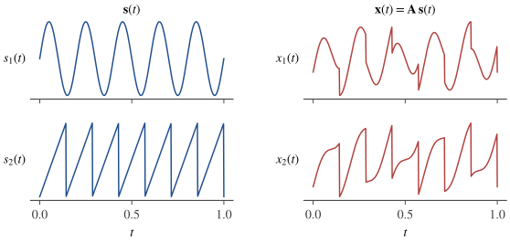
Figure 1.1图 1.1 shows the idea with two synthetic signals. The sources and are a sinusoid and a sawtooth; the sensors observe and , each a weighted sum of the two. Neither recording looks like a clean sinusoid or a clean sawtooth, yet together the two recordings contain everything needed to undo the mixing.
Figure 1.1图 1.1 用两个合成信号说明这一想法。源信号 与 分别是正弦波和锯齿波;传感器观测到 与 ,各自是两个源的加权和。单看任何一段录音,都既不像干净的正弦波,也不像干净的锯齿波;但两段录音合在一起,已经包含了撤销混合所需的全部信息。
The same structure appears whenever several sensors record superpositions of a few underlying processes:
只要若干传感器记录的是少数几个潜在过程的叠加,就会出现同样的结构:
- EEG and MEG. Each scalp electrode or magnetometer records a weighted sum of activity from many brain sources, together with eye blinks, muscle activity and line noise. ICA is routinely used to separate such artifacts from brain signals (Makeig et al., 1996; Jung et al., 2000).
- Functional MRI. Every voxel's time series mixes several spatially distributed processes. Spatial ICA decomposes fMRI data into maps of coherent networks and their time courses (McKeown et al., 1998); Part VI of this book is devoted to it.
- Communications and audio. Antenna arrays receive superpositions of transmitted signals; microphone arrays receive superpositions of voices.
- Natural images. Applied to small patches of natural images, ICA yields localized, oriented filters that resemble the receptive fields of simple cells in primary visual cortex (Bell & Sejnowski, 1997; van Hateren & van der Schaaf, 1998).
- EEG 与 MEG。每个头皮电极或磁强计记录的是许多脑内源活动的加权和,再加上眨眼、肌电和工频干扰。ICA 常被用来把这些伪迹与脑信号分开(Makeig et al., 1996; Jung et al., 2000)。
- 功能磁共振(fMRI)。每个体素的时间序列都混合了若干空间分布的过程。空间 ICA 把 fMRI 数据分解为一组协同网络的空间图及其时间过程(McKeown et al., 1998);本书第六部分专门讨论这一应用。
- 通信与音频。天线阵列接收的是多个发射信号的叠加;麦克风阵列接收的是多个人声的叠加。
- 自然图像。把 ICA 用于自然图像的小块,得到的是局部化、有方向性的滤波器,与初级视皮层简单细胞的感受野相似(Bell & Sejnowski, 1997; van Hateren & van der Schaaf, 1998)。
In each case the sensors see mixtures, the quantities of interest are the unmixed components, and neither the mixing weights nor the components are known in advance. The task is therefore called blind source separation (BSS). ICA is the best-known approach to it, and the subject of this book.
在这些例子里,传感器看到的都是混合,我们关心的是未混合的成分,而混合权重与成分本身事先都不知道。因此这一任务被称为盲源分离(blind source separation, BSS)。ICA 是解决它最著名的方法,也是本书的主题。
Jutten and Hérault (1991) described an early adaptive algorithm for separating sources; Comon (1994) gave ICA a precise formulation and proved that it is identifiable; and the Infomax algorithm of Bell and Sejnowski (1995) brought it into wide use. Hyvärinen, Karhunen and Oja (2001) and Comon and Jutten (2010) give book-length treatments.
Jutten 与 Hérault(1991)描述了一种早期的自适应源分离算法;Comon(1994)给出了 ICA 的严格表述,并证明了它的可辨识性;Bell 与 Sejnowski(1995)的 Infomax 算法使 ICA 得到广泛应用。Hyvärinen、Karhunen 与 Oja(2001)以及 Comon 与 Jutten(2010)是这一领域的专著。
1.2 The linear mixing model线性混合模型
Write the unknown source signals at time as a vector and the observed signals as . The linear instantaneous mixing model states that
把时刻 的 个未知源信号写成向量 ,把 个观测信号写成 。线性瞬时混合模型假设
where is an unknown constant mixing matrix. Column of , written , describes how source reaches the sensors, so (1.1) can also be read as : every observation is a superposition of fixed patterns with time-varying amplitudes . Stacking the samples as columns gives the matrix form , with and .
其中 是未知的常数混合矩阵。 的第 列记为 ,描述源 如何到达各传感器,所以 (1.1) 也可以写成 :每个观测都是若干固定模式 的叠加,叠加系数 随时间变化。把 个样本按列排开,得到矩阵形式 ,其中 ,。
Instantaneous means that each source reaches every sensor at the same moment, without delays or echoes. This holds well for EEG, where electrical fields propagate through the head essentially instantly, and for the spatial ICA of fMRI. It does not hold for speech recorded in a real room, where each microphone receives filtered and delayed copies of the voices (a convolutive mixture); that harder problem lies outside this book.
瞬时指每个源同时到达所有传感器,没有延迟或回声。对 EEG 来说这一假设相当准确,因为电场在头部的传播几乎是瞬时的;fMRI 的空间 ICA 也满足这一点。但在真实房间里录制的语音并不满足:每只麦克风收到的是经过滤波和延迟的声音副本(卷积混合),这个更难的问题不在本书范围之内。
Throughout the book, the model comes with the following standing assumptions, unless a chapter says otherwise.
除非某章另有说明,全书都在以下基本假设下讨论这个模型。
Assumption 1.1 (the standard ICA model)假设 1.1(标准 ICA 模型)
- The sources are mutually statistically independent.
- At most one source is Gaussian.
- The mixing matrix has full column rank ; in particular .
- The samples are independent draws from one distribution, and each source has zero mean and finite, nonzero variance.
- 源 相互统计独立。
- 至多有一个源是高斯的。
- 混合矩阵 列满秩,秩为 ;特别地 。
- 样本 是来自同一分布的独立抽样;各源均值为零,方差有限且不为零。
Independence is the structural heart of the model: the joint density factorizes, . The restriction on Gaussian sources is what makes the problem solvable at all; Chapter 4第 4 章 proves that, together with the other assumptions, it is also enough. Full column rank ensures that no source is lost or confounded with another. Zero means cost nothing: subtract the sample mean of first, and recover the source means afterwards as . Finite variances make the covariance of well defined, and nonzero variances rule out a source that is identically zero, which could be paired with any column of . The i.i.d. assumption means that standard ICA ignores time order entirely; it would give the same answer if the samples were shuffled. Chapter 9第 9 章 shows how temporal structure can be used instead.
独立性是这个模型的结构核心:联合密度可以分解为 。对高斯源个数的限制,是问题能够求解的前提;Chapter 4第 4 章会证明:在其余假设成立时,这一限制也是充分的。列满秩保证没有哪个源丢失或与其他源混淆。零均值不构成任何限制:先减去 的样本均值,最后再用 恢复源的均值即可。方差有限保证 的协方差有定义;方差不为零则排除了恒为零的源,因为这样的源可以与 的任意一列相配。独立同分布假设意味着标准 ICA 完全忽略时间顺序:把样本打乱,结果也不会变。Chapter 9第 9 章会说明如何转而利用时间结构。
Definition 1.2 (independent component analysis)定义 1.2(独立成分分析)
Given samples from the model (1.1), independent component analysis estimates an unmixing matrix such that the components of the output are mutually independent. The matrix , which maps sources to outputs through , is called the global (or gain) matrix.
给定来自模型 (1.1) 的样本 ,独立成分分析估计一个解混矩阵 ,使输出 的各分量相互独立。矩阵 通过 把源映射到输出,称为全局矩阵(或增益矩阵)。
With finite data, exact independence cannot be verified, so in practice is chosen to optimize a contrast function, a statistic that measures how independent or non-Gaussian the outputs are. Chapters 5 and 6 build these contrasts; Part III turns them into algorithms.
在有限数据下无法验证严格的独立性,因此实践中 是通过优化某个对比函数(衡量输出有多独立或多非高斯的统计量)得到的。第 5、6 章构造这些对比函数,第三部分把它们变成算法。
1.3 What cannot be recovered无法恢复的量
Two things are lost in principle, however much data we have. The first is scale, including sign: since for any nonzero numbers , a source can be multiplied by a constant and its column divided by the same constant without changing the observations. The second is order: the sum does not depend on how its terms are numbered, so permuting the sources and the columns of together changes nothing either.
无论数据有多少,有两样东西原则上无法恢复。第一是尺度(包括符号):对任意非零数 ,都有 ,所以把某个源乘以一个常数、同时把对应的列除以同一常数,观测不会改变。第二是顺序:求和与各项的编号无关,因此把源和 的列同时重新排列,观测同样不变。
Proposition 1.3 (scaling and permutation indeterminacy)命题 1.3(尺度与置换不确定性)
Let be an permutation matrix and an invertible diagonal matrix. Then the pair generates exactly the same observations as , and the components of are again mutually independent, with as many Gaussian components as . Consequently no method can do better than to find with , that is, to recover the sources up to order and scale.
设 是 置换矩阵, 是可逆对角矩阵。则 与 生成完全相同的观测,并且 的各分量仍相互独立,所含高斯分量的个数也与 相同。因此任何方法最多只能找到满足 的 ,即在顺序与尺度意义下恢复源。
Proof.证明
Since , we have . The components of are the numbers in a different order; functions of independent random variables taken one at a time remain independent, and a nonzero multiple of a variable is Gaussian exactly when the variable is.
由于 ,有 。 的分量就是重新排序后的 ;对独立随机变量逐个作函数变换,结果仍然独立;而一个变量的非零倍数是高斯的,当且仅当该变量本身是高斯的。
Separation therefore succeeds when the global matrix has exactly one nonzero entry in each row and each column. For instance, with , an algorithm that returns with has succeeded completely: its outputs are and .
因此,当全局矩阵 的每行每列恰有一个非零元时,分离就成功了。例如,对 ,若某算法给出的 满足 ,它就完全成功了:输出为 ,。
In practice the ambiguities are removed by convention. The scale is usually fixed by requiring unit variance, , which leaves only the sign. Signs and order are then fixed by whatever is natural for the application: in fMRI, for example, each spatial map is flipped so that its heavier tail is positive, and components are ordered by explained variance or by a contrast value. How close an estimated is to a scaled permutation, when separation is only approximate, is the subject of Chapter 10第 10 章.
实践中,这些不确定性靠约定来消除。尺度通常通过要求单位方差 来固定,只剩下符号未定。符号与顺序再按应用中自然的方式确定:例如在 fMRI 中,把每张空间图翻转到其较重的尾部为正,并按解释方差或对比函数值给成分排序。当分离只是近似成功时,如何度量估计的 离带尺度的置换矩阵有多近,是Chapter 10第 10 章的主题。
1.4 Why not PCA or factor analysis?为什么不用 PCA 或因子分析?
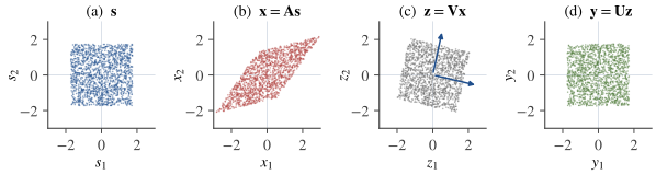
Principal component analysis (PCA) finds an orthogonal transform that makes the outputs uncorrelated and orders them by variance. If were orthogonal and the source variances were distinct, PCA would recover the sources up to sign. In general, however, is not orthogonal, and being uncorrelated is a much weaker requirement than being independent. Figure 1.2图 1.2 makes the difference visible. Two uniform sources fill a square (a). Mixing shears the square into a parallelogram (b). Whitening, for example PCA followed by rescaling each principal component to unit variance, turns the parallelogram back into a square, but leaves it rotated by an unknown angle (c; the figure uses the symmetric whitening matrix , see Chapter 3第 3 章). Only by using information beyond the covariance does ICA find the rotation that aligns the square with the axes (d).
主成分分析(PCA)寻找一个正交变换,使输出互不相关并按方差排序。如果 是正交矩阵、且各源方差互不相同,PCA 能在符号意义下恢复源。但一般情况下 并不正交,而且不相关是比独立弱得多的要求。Figure 1.2图 1.2 直观地展示了两者的差别。两个均匀分布的源填满一个正方形(a)。混合把正方形剪切成平行四边形(b)。白化(例如先做 PCA、再把每个主成分缩放到单位方差)会把平行四边形变回正方形,但这个正方形转过了一个未知的角度(c;图中使用的是对称白化矩阵 ,见Chapter 3第 3 章)。只有利用协方差之外的信息,ICA 才能找到把正方形摆正的那个旋转(d)。
A count of parameters shows why the covariance cannot be enough. Take and unit-variance sources. The covariance is symmetric, so it supplies numbers, while has unknown entries. The shortfall is , which is exactly the number of free parameters of an orthogonal matrix: any with orthogonal has the same covariance as . Second-order statistics determine the mixing matrix only up to a rotation. Chapter 3第 3 章 makes this precise, and Chapter 4第 4 章 shows that higher-order statistics pin down the rotation as soon as the sources are non-Gaussian.
数一数参数,就能看出为什么协方差不够用。取 且源为单位方差。协方差 是对称矩阵,只提供 个数,而 有 个未知元。两者相差 ,恰好是一个 正交矩阵的自由参数个数:对任意正交矩阵 , 与 有相同的协方差。二阶统计量只能把混合矩阵确定到一个旋转。Chapter 3第 3 章会把这一点说清楚,Chapter 4第 4 章则证明:只要源是非高斯的,高阶统计量就能确定这个旋转。
Gaussian sources are the exception. If , then has exactly the same distribution as for every orthogonal , so the data cannot distinguish from by any statistic whatsoever. This is why the standard model allows at most one Gaussian source. Classical factor analysis meets the same obstruction: it models with Gaussian factors , so its loadings are determined only up to rotation, and heuristics such as varimax are needed to choose one. ICA can be read as factor analysis with non-Gaussian independent factors, the assumption that removes the rotational freedom.
高斯源是例外。若 ,则对任意正交矩阵 , 与 的分布完全相同,因此任何统计量都无法从数据中区分 与 。这就是标准模型至多允许一个高斯源的原因。经典的因子分析遇到的是同一障碍:它的模型是 ,因子 为高斯分布,所以载荷矩阵只能确定到一个旋转,需要 varimax 之类的启发式方法来选定一个。可以把 ICA 理解为因子相互独立且非高斯的因子分析,正是这一假设消除了旋转自由度。
1.5 A first look at how ICA works初窥 ICA 的工作方式
Most ICA methods follow the two-step logic of Figure 1.2图 1.2. First, whiten: find a matrix such that has identity covariance. What remains is to find an orthogonal such that has independent components, a search over rotations. Second, choose the rotation with a contrast function that measures non-Gaussianity or independence. The intuition is the central limit theorem: a sum of independent variables tends to be more Gaussian than the variables themselves, so a mixture of several sources is typically more Gaussian than the most non-Gaussian of them. Making each output as non-Gaussian as possible therefore drives it toward one source; Chapter 5第 5 章 turns this intuition into a theorem.
大多数 ICA 方法都遵循 Figure 1.2图 1.2 所示的两步思路。第一步是白化:找一个矩阵 ,使 的协方差为单位阵。剩下的任务是找一个正交矩阵 ,使 的分量相互独立,也就是在旋转中搜索。第二步是用对比函数来选择旋转,对比函数衡量的是非高斯性或独立性。其直觉来自中心极限定理:独立变量之和往往比各个变量本身更接近高斯,所以几个源的混合通常比其中最非高斯的那个源更接近高斯。让每个输出尽可能非高斯,就会把它推向某一个源;Chapter 5第 5 章会把这一直觉变成定理。
The following script carries out both steps for two sources, one uniform and one Laplacian, using kurtosis (the fourth cumulant, ) as the contrast and a brute-force search over the rotation angle.
下面的脚本对两个源(一个均匀分布、一个拉普拉斯分布)完成这两步,用峭度(四阶累积量,)作为对比函数,并对旋转角做穷举搜索。
import numpy as np

rng = np.random.default_rng(0)
T = 5000
S = np.vstack([rng.uniform(-np.sqrt(3), np.sqrt(3), T),   # uniform: sub-Gaussian, unit variance
               rng.laplace(0.0, 1 / np.sqrt(2), T)])      # Laplace: super-Gaussian, unit variance
A = np.array([[1.0, 0.6],
              [0.4, 1.0]])
X = A @ S                                    # observed mixtures, shape (2, T)

# Step 1: whiten, z = V x with sample covariance I
X = X - X.mean(axis=1, keepdims=True)
d, E = np.linalg.eigh(np.cov(X))
V = E @ np.diag(d ** -0.5) @ E.T
Z = V @ X

# Step 2: rotate, choosing the direction whose projection has the largest |kurtosis|
def kurt(y):
    return np.mean(y ** 4) - 3 * np.mean(y ** 2) ** 2

angles = np.linspace(0, np.pi, 360, endpoint=False)
scores = [abs(kurt(np.cos(a) * Z[0] + np.sin(a) * Z[1])) for a in angles]
a = angles[np.argmax(scores)]
U = np.array([[np.cos(a), np.sin(a)],
              [-np.sin(a), np.cos(a)]])
Y = U @ Z                                    # estimated sources
W = U @ V                                    # estimated unmixing matrix
print(np.round(W @ A, 2))                    # close to a signed permutation
On this run the script prints : the first output is the Laplacian source and the second is the uniform source with its sign flipped, exactly the ambiguity that Proposition 1.3命题 1.3 allows. Directions and give the same projection up to sign, so searching angles in covers every direction once. A brute-force search works only in two dimensions; Chapters 7 to 9 develop algorithms that scale to many sources, and Chapter 10第 10 章 asks how accurate any algorithm can possibly be.
这次运行输出 :第一个输出是拉普拉斯源,第二个输出是符号翻转后的均匀源,恰好是Proposition 1.3命题 1.3所允许的不确定性。方向 与 给出的投影只差一个符号,所以在 内搜索角度恰好覆盖每个方向一次。穷举搜索只在二维可行;第 7 至 9 章发展能处理大量源的算法,Chapter 10第 10 章则讨论任何算法最多能达到多高的精度。
1.6 How this book is organized本书的结构
The book has six parts and an appendix. Each chapter ends with exercises at three levels (basic, intermediate and advanced) with solutions that open on request.
本书分为六个部分和一个附录。每章末尾都有三个难度级别(基础、进阶、硬核)的习题,解答默认折叠,点开即可查看。
- Part I. Foundations
- This chapter; the probability tools of ICA (Chapter 2第 2 章); whitening and the geometry of the problem (Chapter 3第 3 章).
- Part II. Principles
- Identifiability (Chapter 4第 4 章); non-Gaussianity and kurtosis (Chapter 5第 5 章); negentropy, mutual information and likelihood (Chapter 6第 6 章).
- Part III. Algorithms
- Natural gradient and Infomax (Chapter 7第 7 章); FastICA (Chapter 8第 8 章); JADE and second-order methods (Chapter 9第 9 章).
- Part IV. Statistical theory
- Asymptotic performance and the Cramér–Rao bound (Chapter 10第 10 章); noise, model order and reliability (Chapter 11第 11 章).
- Part V. Beyond the square linear model
- Overcomplete ICA (Chapter 12第 12 章); nonlinear ICA (Chapter 13第 13 章).
- Part VI. ICA for brain imaging
- Spatial ICA of fMRI (Chapter 14第 14 章); group ICA, dual regression and IVA (Chapter 15第 15 章).
- 第一部分:基础
- 本章;ICA 的概率工具(Chapter 2第 2 章);白化与问题的几何(Chapter 3第 3 章)。
- 第二部分:原理
- 可辨识性(Chapter 4第 4 章);非高斯性与峭度(Chapter 5第 5 章);负熵、互信息与似然(Chapter 6第 6 章)。
- 第三部分:算法
- 自然梯度与 Infomax(Chapter 7第 7 章);FastICA(Chapter 8第 8 章);JADE 与二阶方法(Chapter 9第 9 章)。
- 第四部分:统计理论
- 渐近性能与 Cramér–Rao 界(Chapter 10第 10 章);噪声、模型阶数与可靠性(Chapter 11第 11 章)。
- 第五部分:超越方阵线性模型
- 过完备 ICA(Chapter 12第 12 章);非线性 ICA(Chapter 13第 13 章)。
- 第六部分:脑影像中的 ICA
- fMRI 的空间 ICA(Chapter 14第 14 章);组 ICA、双回归与独立向量分析(Chapter 15第 15 章)。
Two reading paths work well. For practice, read Chapters 1, 3, 5 and 8 and then Part VI. For theory, read Parts I and II in order, then Chapters 7, 10, 12 and 13. Appendix A附录 A collects the facts from matrix analysis, optimization and asymptotic statistics used throughout.
推荐两条阅读路线。偏重应用:读第 1、3、5、8 章,然后读第六部分。偏重理论:按顺序读第一、二部分,再读第 7、10、12、13 章。Appendix A附录 A汇集了全书用到的矩阵分析、优化与渐近统计知识。
1.7 Notation记号
Vectors are bold lowercase, matrices bold uppercase, scalars italic. All vectors are column vectors, and denotes transposition. The symbols below keep the same meaning in every chapter unless a chapter says otherwise; Part VI, for example, writes fMRI data as a matrix with time points and voxels.
向量用粗体小写字母,矩阵用粗体大写字母,标量用斜体。所有向量都是列向量, 表示转置。除非某章另有说明,下表中的记号在全书各章含义不变;例如第六部分把 fMRI 数据写成 个时间点 × 个体素的矩阵。
| Symbol记号 | Meaning含义 |
|---|---|
| numbers of sources, sensors and samples源、传感器与样本的个数 | |
| source vector, with densities of 源向量, 的密度为 | |
| observations, mixing matrix, its -th column观测、混合矩阵及其第 列 | |
| unmixing matrix and its outputs解混矩阵及其输出 | |
| global (gain) matrix全局(增益)矩阵 | |
| whitening matrix, whitened data, whitened mixing matrix白化矩阵、白化数据、白化后的混合矩阵 | |
| orthogonal matrices (the rotation found after whitening; a generic one)正交矩阵(白化后求出的旋转;一般的正交矩阵) | |
| permutation, diagonal and identity matrices置换矩阵、对角矩阵、单位矩阵 | |
| expectation, sample average, covariance of zero-mean 期望、样本平均、零均值 的协方差 | |
| one-unit methods: a unit vector, its projection, and the same direction in source coordinates单单元方法:单位向量、其投影,以及同一方向在源坐标下的表示 | |
| score function of source 源 的得分函数 | |
| Fisher information of the unit-variance source (, with equality only for a Gaussian)单位方差源 的 Fisher 信息(,仅当源为高斯时取等号) | |
| nonlinearity of gradient algorithms; nonlinearity of FastICA梯度算法中的非线性函数;FastICA 中的非线性函数 | |
| kurtosis, cumulant峭度、累积量 | |
| kurtosis of the unit-variance source 单位方差源 的峭度 | |
| a standard Gaussian variable, 标准高斯变量, | |
| differential entropy, negentropy, mutual information, Kullback–Leibler divergence微分熵、负熵、互信息、KL 散度 | |
| Gaussian distribution高斯分布 |
Key points
本章要点
- ICA models observations as an instantaneous linear mixture of independent sources and estimates an unmixing matrix .
- The scale, sign and order of the sources can never be recovered; success means that is a scaled permutation matrix.
- Second-order statistics determine only up to a rotation; independence and non-Gaussianity determine the rotation.
- Gaussian sources are the exception: among two or more Gaussian sources, no rotation can be told apart from another.
- ICA 把观测建模为独立源的瞬时线性混合 ,并估计解混矩阵 。
- 源的尺度、符号与顺序永远无法恢复;分离成功意味着 是带尺度的置换矩阵。
- 二阶统计量只能把 确定到一个旋转;独立性与非高斯性确定这个旋转。
- 高斯源是例外:两个及以上高斯源之间,任何旋转都无法区分。
1.8 Exercises习题
Exercise 1.1习题 1.1 basic基础
Suppose separates the mixture exactly, . Show that also produces mutually independent outputs for every permutation matrix and invertible diagonal matrix . What is ?
设 恰好完成分离,即 。证明对任意置换矩阵 和可逆对角矩阵 , 的输出也相互独立。 等于什么?
Show solution查看解答
, so . Its components are the numbers in a different order: each is a function of a single source, and the sources involved are distinct, so the components are independent.
,所以 。它的分量就是重新排序后的 :每个分量只是某一个源的函数,且涉及的源各不相同,所以这些分量相互独立。
Exercise 1.3习题 1.3 intermediate进阶
Let in and let be any orthogonal matrix. Show that has the same distribution as , and conclude that the observations cannot distinguish the mixing matrix from .
设 取值于 , 是任意 正交矩阵。证明 与 同分布,并由此说明观测 无法区分混合矩阵 与 。
Show solution查看解答
A linear transform of a Gaussian vector is Gaussian, so is Gaussian with mean and covariance ; a Gaussian distribution is determined by its mean and covariance, so . Now , and is again a vector of independent standard Gaussian sources. The models and therefore produce identically distributed observations, and no statistic of can tell them apart.
高斯向量的线性变换仍是高斯的,所以 是均值为 、协方差为 的高斯向量;高斯分布由均值和协方差唯一确定,因此 。又 ,而 仍是由独立标准高斯源组成的向量。于是模型 与 产生同分布的观测,任何关于 的统计量都无法区分它们。
Exercise 1.4习题 1.4 intermediate进阶
For a square model () with unit-variance sources, count the numbers determined by the covariance and the unknowns in . Show that the difference equals the number of free parameters of an orthogonal matrix, and that every matrix with orthogonal has the same covariance.
对方阵模型()且源为单位方差的情形,数一数协方差 确定了多少个数, 又有多少个未知量。证明二者之差等于 正交矩阵的自由参数个数,并且对任意正交矩阵 , 都有相同的协方差。
Show solution查看解答
is symmetric, so it has distinct entries, while has . The difference is . The orthogonality constraints are equations (again by symmetry) on entries, leaving free parameters: one angle for , three for . Finally .
是对称矩阵,只有 个不同的元素,而 有 个元素,两者相差 。正交性约束 同样由于对称性只给出 个方程,作用在 个元素上,剩下 个自由参数: 时是一个角度, 时是三个。最后,。
Exercise 1.5习题 1.5 basic基础
Run the script of Section 1.5第 1.5 节 with both sources replaced by standard Gaussian noise, and plot the absolute kurtosis of the first output against the angle. What do you observe, and why?
把Section 1.5第 1.5 节中脚本的两个源都换成标准高斯噪声,画出第一个输出的峭度绝对值随角度变化的曲线。你观察到什么?为什么?
Show solution查看解答
The curve fluctuates near zero with no consistent peak, and the selected angle changes from one random seed to the next. Every projection of a whitened Gaussian vector is again standard Gaussian, with zero kurtosis, so the estimated kurtosis reflects only sampling noise, of order for . Separation fails, as Exercise 1.3习题 1.3 predicts.
曲线在零附近随机起伏,没有稳定的峰值,选出的角度随随机种子而变。白化后的高斯向量在任意方向上的投影仍是标准高斯分布,峭度为零,因此估计出的峭度只反映抽样噪声,量级约为 ,当 时约为 。分离失败,正如Exercise 1.3习题 1.3所预言的那样。
Exercise 1.6习题 1.6 advanced硬核
Let be independent with zero mean, unit variance and kurtoses , not both zero. Let , where is a rotation, and for the unit vector let . (a) Show that . (b) Show that , with equality only when for a source whose is the larger of the two. (c) The script of Section 1.5第 1.5 节 picks the first output by maximizing over the angle, and its sources have kurtoses (Laplace) and (uniform). Explain why its first output is the Laplacian source and its second output the uniform one.
设 独立,均值为零、方差为一,峭度 不全为零。令 ,其中 是一个旋转;对单位向量 ,令 。(a)证明 。(b)证明 ,且等号只在 时成立,其中源 的 是两者中较大的那个。(c)Section 1.5第 1.5 节的脚本通过对角度最大化 来选出第一个输出,它的两个源的峭度分别为 (拉普拉斯)与 (均匀)。解释为什么第一个输出是拉普拉斯源,第二个输出是均匀源。
Show solution查看解答
(a) Multiplying out, with and , so and . Expanding , the terms with an odd power of a zero-mean source vanish by independence, leaving . Subtracting gives . (b) Let . Then . Equality in the last step forces , that is or , where equals or ; so the maximum is reached exactly at the source with the larger (at both sources if ). (c) The whitened mixing matrix is orthogonal, so the same computation applies to it (a reflection only changes the sign of , which does not affect ). Since , the largest is reached only at the Laplacian source, so the first row of picks it out. The second row of is orthogonal to the first, so in source coordinates it points along the other source: the second output is the uniform source. With the standard errors of the kurtosis estimates, about for the Laplacian source and for the uniform one (over 400 repetitions of the script), are small compared with the gap between and ; the run above gives and .
(a)直接相乘,,其中 ,,所以 ,且 。展开 ,由独立性,含零均值源奇数次幂的项都为零,剩下 。减去 ,得 。(b)记 。则 。最后一步取等号要求 ,即 或 ,此时 分别等于 或 ;所以最大值 恰好在 较大的那个源(的正负号)处取到(若 ,则两个源处都取到)。(c)白化后的混合矩阵 是正交矩阵,上面的计算同样适用(若它是反射,只会改变 的符号,不影响 )。由于 , 的最大值只在 等于正负拉普拉斯源时取到,所以 的第一行挑出了拉普拉斯源。 的第二行与第一行正交,在源坐标下指向另一个源,所以第二个输出是正负均匀源。 时,峭度估计的标准误对拉普拉斯源约为 ,对均匀源约为 (把脚本重复运行 400 次得到),与 和 之间的差距相比都很小;上面那次运行得到的是 与 。
1.9 References参考文献
- Bell, A. J., & Sejnowski, T. J. (1995). An information-maximization approach to blind separation and blind deconvolution. Neural Computation, 7(6), 1129–1159.
- Bell, A. J., & Sejnowski, T. J. (1997). The “independent components” of natural scenes are edge filters. Vision Research, 37(23), 3327–3338.
- Cherry, E. C. (1953). Some experiments on the recognition of speech, with one and with two ears. Journal of the Acoustical Society of America, 25(5), 975–979.
- Comon, P. (1994). Independent component analysis, a new concept? Signal Processing, 36(3), 287–314.
- Comon, P., & Jutten, C. (Eds.) (2010). Handbook of Blind Source Separation: Independent Component Analysis and Applications. Academic Press.
- Hyvärinen, A., Karhunen, J., & Oja, E. (2001). Independent Component Analysis. Wiley.
- Jung, T.-P., Makeig, S., Humphries, C., Lee, T.-W., McKeown, M. J., Iragui, V., & Sejnowski, T. J. (2000). Removing electroencephalographic artifacts by blind source separation. Psychophysiology, 37(2), 163–178.
- Jutten, C., & Hérault, J. (1991). Blind separation of sources, part I: An adaptive algorithm based on neuromimetic architecture. Signal Processing, 24(1), 1–10.
- Makeig, S., Bell, A. J., Jung, T.-P., & Sejnowski, T. J. (1996). Independent component analysis of electroencephalographic data. In Advances in Neural Information Processing Systems 8 (pp. 145–151). MIT Press.
- McKeown, M. J., Makeig, S., Brown, G. G., Jung, T.-P., Kindermann, S. S., Bell, A. J., & Sejnowski, T. J. (1998). Analysis of fMRI data by blind separation into independent spatial components. Human Brain Mapping, 6(3), 160–188.
- van Hateren, J. H., & van der Schaaf, A. (1998). Independent component filters of natural images compared with simple cells in primary visual cortex. Proceedings of the Royal Society B, 265(1394), 359–366.