Non-Gaussianity and Kurtosis非高斯性与峭度

5.1 Mixing makes signals more Gaussian混合使信号更接近高斯

Section 1.5第 1.5 节 separated two sources by choosing the projection of the whitened data with the largest absolute kurtosis. The reasoning was a heuristic drawn from the central limit theorem: a sum of independent variables tends to be more Gaussian than the variables themselves, so a projection that mixes several sources looks more Gaussian than a projection that equals one source, and the least Gaussian projections should be the sources. Chapter 4第 4 章 showed that the sources are determined by the distribution of the data; this chapter shows that, for kurtosis, the heuristic is a theorem, and then examines what the theorem costs in practice.

Section 1.5第 1.5 节选取白化数据中峭度绝对值最大的投影，把两个源分离了出来。其理由是来自中心极限定理的启发式论证：独立变量之和往往比各个变量本身更接近高斯，所以混合了多个源的投影比恰好等于某一个源的投影更像高斯，而最不像高斯的投影就应该是源。Chapter 4第 4 章证明了源由数据的分布唯一确定；本章说明，对峭度而言，这个启发式论证是一个定理，然后再考察这个定理在实践中要付出什么代价。

ICA usually involves a handful of sources, so the limit theorem itself is not what matters. What matters is a statement for finitely many terms: a combination of independent sources sits, in a precise sense, between the sources and the Gaussian. For kurtosis the statement is simple. If $s_1, \dots, s_n$ are independent with unit variance and the same kurtosis $\kappa$, then their normalized sum $n^{-1/2}\sum_i s_i$ has kurtosis $\kappa/n$, and no unit-variance combination has kurtosis larger in absolute value than the most kurtotic source (Proposition 5.1命题 5.1). The analogous statement for entropy is taken up in Chapter 6第 6 章.

ICA 通常只涉及少数几个源，所以要紧的并不是极限定理本身，而是一个关于有限项的论断：独立源的组合在确切的意义上介于源与高斯之间。对峭度而言，这个论断很简单。若 $s_1, \dots, s_n$ 独立、方差为一且峭度同为 $\kappa$，则其归一化和 $n^{-1/2}\sum_i s_i$ 的峭度为 $\kappa/n$；并且任何单位方差的组合，其峭度的绝对值都不会超过峭度最大的那个源（Proposition 5.1命题 5.1）。熵的相应论断留到Chapter 6第 6 章讨论。

Throughout the chapter the data are whitened, $\bz = \tilde\bA\bs$, with $\tilde\bA$ orthogonal and independent zero-mean sources of unit variance and finite fourth moments ((3.2)). A one-unit method looks for a unit vector $\bw$ such that $y = \bw^\top\bz$ is a source. In source coordinates, $\bq = \tilde\bA^\top\bw$, the projection is $y = \bq^\top\bs$, and $\|\bq\| = \|\bw\| = 1$ because $\tilde\bA$ is orthogonal; in particular $\E[y^2] = \|\bq\|^2 = 1$. Searching over unit vectors $\bw$ is therefore the same as searching over unit vectors $\bq$, and $y$ is a source exactly when $\bq = \pm\be_i$, a standard basis vector.

本章始终假定数据已经白化：$\bz = \tilde\bA\bs$，其中 $\tilde\bA$ 是正交矩阵，各源独立、均值为零、方差为一且四阶矩有限（(3.2)）。单单元方法寻找一个单位向量 $\bw$，使 $y = \bw^\top\bz$ 是某个源。在源坐标 $\bq = \tilde\bA^\top\bw$ 下，投影为 $y = \bq^\top\bs$；由于 $\tilde\bA$ 正交，$\|\bq\| = \|\bw\| = 1$，特别地 $\E[y^2] = \|\bq\|^2 = 1$。因此在单位向量 $\bw$ 上搜索，等价于在单位向量 $\bq$ 上搜索；而 $y$ 恰为某个源，当且仅当 $\bq = \pm\be_i$ 是标准基向量。

The same idea appeared earlier in exploratory statistics as projection pursuit. Friedman & Tukey (1974) proposed to explore multivariate data by numerically optimizing a "projection index" over one- or two-dimensional projections. Huber (1985) argued that the Gaussian is the least interesting distribution, since most projections of high-dimensional data look nearly Gaussian, so that a projection index should measure departure from Gaussianity. One-unit ICA contrasts are projection indices of exactly this kind, applied to whitened data; under the ICA model the interesting directions are the sources (Hyvärinen, Karhunen & Oja, 2001).

同样的思想更早出现在探索性统计中，名为投影寻踪。Friedman & Tukey（1974）提出，在一维或二维投影上数值优化一个“投影指标”，以此探索多元数据。Huber（1985）认为高斯分布是最没有意思的分布，因为高维数据的大多数投影看上去都近似高斯，所以投影指标应当度量偏离高斯的程度。单单元 ICA 对比函数正是这类投影指标，只不过作用在白化数据上；在 ICA 模型下，有意思的方向就是源（Hyvärinen, Karhunen & Oja, 2001）。

5.2 Kurtosis of a linear combination线性组合的峭度

For a zero-mean variable, $\kurt(y) = \E[y^4] - 3(\E[y^2])^2$ is the fourth cumulant (Definition 2.10定义 2.10). It vanishes for the Gaussian; variables with $\kurt(y) < 0$ are called sub-Gaussian (uniform: $-1.2$; a binary $\pm 1$ variable: $-2$, the smallest possible value at unit variance) and variables with $\kurt(y) > 0$ super-Gaussian (Laplace: $3$; centered exponential: $6$). As a cumulant it has two properties that drive everything in this chapter: for independent $u$ and $v$ and a real number $\alpha$,

对零均值变量，$\kurt(y) = \E[y^4] - 3(\E[y^2])^2$ 就是四阶累积量（Definition 2.10定义 2.10）。高斯变量的峭度为零；$\kurt(y) < 0$ 的变量称为亚高斯的（均匀分布为 $-1.2$；取 $\pm 1$ 的二值变量为 $-2$，这是单位方差下可能取到的最小值），$\kurt(y) > 0$ 的变量称为超高斯的（拉普拉斯分布为 $3$；中心化的指数分布为 $6$）。作为累积量，它有两条性质，本章的一切都由它们推出：对独立的 $u$、$v$ 与实数 $\alpha$，

Three consequences shape the rest of the chapter. First, mixing can never produce more absolute kurtosis than the most kurtotic source contains, which is the precise form of the central-limit heuristic. Second, a mixture can still be more kurtotic than some of the sources: mixing a nearly Gaussian source with a Laplacian one gives a combination that is less Gaussian than the first source. Third, kurtoses of opposite signs can cancel: for a uniform and a Laplacian source, $\kurt(\cos\theta\, s_1 + \sin\theta\, s_2) = -1.2\cos^4\theta + 3\sin^4\theta$ vanishes at $\tan^4\theta = 0.4$, that is $\theta \approx 38.5^\circ$, although this combination is certainly not Gaussian. Kurtosis is a signed measure, and the quantities to maximize are $|\kurt|$ or $\kurt^2$.

由此得到的三点决定了本章其余部分。其一，混合产生的峭度绝对值永远不会超过峭度最大的源，这正是中心极限启发式论证的精确形式。其二，混合仍可能比某些源的峭度更大：把一个接近高斯的源与一个拉普拉斯源混合，得到的组合比前者更不像高斯。其三，符号相反的峭度会相互抵消：对一个均匀源和一个拉普拉斯源，$\kurt(\cos\theta\, s_1 + \sin\theta\, s_2) = -1.2\cos^4\theta + 3\sin^4\theta$ 在 $\tan^4\theta = 0.4$，即 $\theta \approx 38.5^\circ$ 处为零，而这个组合显然不是高斯的。峭度是带符号的量，应当最大化的是 $|\kurt|$ 或 $\kurt^2$。

5.3 The kurtosis landscape on the sphere峭度在球面上的地形

By Proposition 5.1命题 5.1, the one-unit contrast in source coordinates is the quartic form $F(\bq) = \sum_i \kappa_i q_i^4$ restricted to the unit sphere, and $|\kurt(\bw^\top\bz)| = |F(\tilde\bA^\top\bw)|$. The map $\bw \mapsto \tilde\bA^\top\bw$ is an isometry of the sphere, so local maxima in $\bw$ and in $\bq$ correspond. The global maximum of $|F|$ sits at a source with the largest $|\kappa_i|$. The question that matters for algorithms, which climb from a random starting point, is whether $|F|$ has other local maxima. We first find all critical points of $F$ on the sphere (see Section A.7第 A.7 节 for the Lagrange conditions).

由Proposition 5.1命题 5.1，在源坐标下，单单元对比函数就是限制在单位球面上的四次型 $F(\bq) = \sum_i \kappa_i q_i^4$，且 $|\kurt(\bw^\top\bz)| = |F(\tilde\bA^\top\bw)|$。映射 $\bw \mapsto \tilde\bA^\top\bw$ 是球面的等距变换，所以 $\bw$ 与 $\bq$ 中的局部极大点一一对应。$|F|$ 的全局最大值出现在 $|\kappa_i|$ 最大的源处。对从随机起点出发向上爬的算法来说，真正要紧的问题是：$|F|$ 还有没有别的局部极大点？我们先求出 $F$ 在球面上的全部临界点（拉格朗日条件见Section A.7第 A.7 节）。

Every single-source point $\pm\be_i$ is critical, with $\mu = \kappa_i$. The critical points with $|S| \ge 2$ mix sources whose kurtoses share a sign, with weights $q_i^2 \propto 1/\kappa_i$; the theorem below shows that none of them is a local maximum of $|F|$.

每个单源点 $\pm\be_i$ 都是临界点，对应 $\mu = \kappa_i$。$|S| \ge 2$ 的临界点则把峭度同号的若干个源混合在一起，权重为 $q_i^2 \propto 1/\kappa_i$；下面的定理说明，它们没有一个是 $|F|$ 的局部极大点。

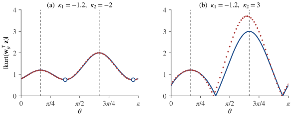
Figure 5.1图 5.1 shows the landscape for two sources. With two sub-Gaussian sources (a), $|\kurt|$ has its local maxima at the two source directions and local minima at the interior critical points, where $\tan^2(\theta - \theta_0) = \kappa_1/\kappa_2$ and $|\kurt| = |(1/\kappa_1 + 1/\kappa_2)^{-1}| = 0.75$. With a sub- and a super-Gaussian source (b), there are no interior critical points with $|S| = 2$; instead the kurtosis changes sign between the source directions, and $|\kurt|$ drops to zero. In both cases every local maximum is a source, as the theorem says.

Figure 5.1图 5.1展示了两个源时的地形。两个源都是亚高斯时（a），$|\kurt|$ 的局部极大点位于两个源方向，局部极小点位于内部临界点，在那里 $\tan^2(\theta - \theta_0) = \kappa_1/\kappa_2$，$|\kurt| = |(1/\kappa_1 + 1/\kappa_2)^{-1}| = 0.75$。一个亚高斯源加一个超高斯源时（b），不存在 $|S| = 2$ 的内部临界点；峭度在两个源方向之间改变符号，$|\kurt|$ 降到零。两种情形下，每个局部极大点都是源，正如定理所言。

Two practical remarks follow. First, the absolute value matters. Maximizing $\kurt$ itself finds super-Gaussian sources, but if all sources are sub-Gaussian then $F < 0$ everywhere and its maximum is the critical point with the largest $\mu$, which is the one with full support: the direction that mixes all sources (Exercise 5.2习题 5.2). An algorithm must either maximize $|\kurt|$ or $\kurt^2$, or know the sign of the kurtosis it is looking for. Second, a source with $\kappa_i = 0$ produces no local maximum at all: kurtosis cannot see it, even if it is far from Gaussian. We return to this in Section 5.6第 5.6 节.

由此得到两点实际的提醒。第一，绝对值不能省。直接最大化 $\kurt$ 能找到超高斯源；但若所有源都是亚高斯的，则 $F$ 处处为负，其最大值落在 $\mu$ 最大的临界点，也就是支撑集为全集的那个点：把所有源混在一起的方向（Exercise 5.2习题 5.2）。算法要么最大化 $|\kurt|$ 或 $\kurt^2$，要么事先知道所找峭度的符号。第二，$\kappa_i = 0$ 的源根本不产生局部极大点：即使它远离高斯，峭度也看不见它。我们将在Section 5.6第 5.6 节回到这一点。

5.4 All components at once: Comon's contrast同时估计全部成分：Comon 对比函数

One-unit methods find the sources one at a time. To estimate all of them together, search over orthogonal matrices $\bU$, with outputs $\by = \bU\bz$, and add up a one-unit contrast over the outputs. Comon (1994) proposed the sum of squared kurtoses,

单单元方法一次只找一个源。若要同时估计全部源，可以在正交矩阵 $\bU$ 上搜索，输出为 $\by = \bU\bz$，并把单单元对比函数对各个输出求和。Comon（1994）提出了峭度平方和

For outputs that are symmetric and close to Gaussian, maximizing $\Psi$ approximately minimizes their mutual information (Section 6.7第 6.7 节). With the orthogonal matrix $\bQ = \bU\tilde\bA$ we have $\by = \bQ\bs$, and by Proposition 5.1命题 5.1, $\kurt(y_i) = \sum_j Q_{ij}^4 \kappa_j$.

对于对称且接近高斯的输出，最大化 $\Psi$ 近似于最小化输出的互信息（Section 6.7第 6.7 节）。记正交矩阵 $\bQ = \bU\tilde\bA$，则 $\by = \bQ\bs$，并由Proposition 5.1命题 5.1得 $\kurt(y_i) = \sum_j Q_{ij}^4 \kappa_j$。

Unlike the one-unit contrast, $\Psi$ tolerates one source with zero kurtosis. It also has a useful interpretation. The sum of the squares of all fourth-order cumulants of $\by$, $\sum_{ijkl}\cum(y_i, y_j, y_k, y_l)^2$, does not depend on the rotation and equals $\sum_j \kappa_j^2$ (Exercise 5.6习题 5.6). Maximizing the diagonal part $\Psi$ is therefore the same as minimizing the sum of the squared cross-cumulants, which is the idea behind JADE (Chapter 9第 9 章).

与单单元对比函数不同，$\Psi$ 能容忍一个峭度为零的源。它还有一个有用的解释：$\by$ 的全部四阶累积量的平方和 $\sum_{ijkl}\cum(y_i, y_j, y_k, y_l)^2$ 与旋转无关，恒等于 $\sum_j \kappa_j^2$（Exercise 5.6习题 5.6）。因此最大化对角部分 $\Psi$，等价于最小化交叉累积量的平方和，这正是 JADE 的思路（Chapter 9第 9 章）。

5.5 Gradient ascent, a fixed point, and deflation梯度上升、不动点与逐个提取

Gradient ascent. For whitened data $\E[(\bw^\top\bz)^2] = \|\bw\|^2$, so $\kurt(\bw^\top\bz) = \E[(\bw^\top\bz)^4] - 3\|\bw\|^4$ and

梯度上升。对白化数据有 $\E[(\bw^\top\bz)^2] = \|\bw\|^2$，所以 $\kurt(\bw^\top\bz) = \E[(\bw^\top\bz)^4] - 3\|\bw\|^4$，且

To increase $|\kurt|$, take a step along the gradient multiplied by the sign of the current kurtosis, then renormalize. The second term of the gradient points along $\bw$; after normalization it only rescales the step, so it can be dropped:

为了增大 $|\kurt|$，沿梯度乘以当前峭度的符号走一步，再归一化。梯度的第二项沿 $\bw$ 方向，归一化之后只改变步长，因此可以略去：

With the expectation replaced by a sample average this is a batch algorithm; with one sample per step it is a stochastic (online) algorithm. Because $|\kurt|$ has no local maxima other than the sources (Theorem 5.3定理 5.3), gradient ascent with a small step size cannot be trapped at a spurious maximum. Its costs are a step size $\mu$ that must be tuned and only linear convergence.

把期望换成样本平均，就得到批处理算法；每一步只用一个样本，就得到随机（在线）算法。由于 $|\kurt|$ 除源方向外没有其他局部极大点（Theorem 5.3定理 5.3），步长足够小的梯度上升不会被困在伪极大点。它的代价是需要调节步长 $\mu$，而且只有线性收敛速度。

A fixed-point iteration. At a critical point on the sphere the gradient (5.4) is parallel to $\bw$, so $\E[\bz(\bw^\top\bz)^3] - 3\bw$ is a multiple of $\bw$. Hyvärinen & Oja (1997) turned this condition into an iteration without a step size:

不动点迭代。在球面上的临界点处，梯度 (5.4) 与 $\bw$ 平行，所以 $\E[\bz(\bw^\top\bz)^3] - 3\bw$ 是 $\bw$ 的倍数。Hyvärinen & Oja（1997）把这个条件变成了一个无需步长的迭代：

In source coordinates the iteration is strikingly simple. For a unit vector $\bq$, expand $\E[s_i(\bq^\top\bs)^3] = \sum_{j,k,l} q_j q_k q_l \E[s_i s_j s_k s_l]$. By independence and zero means only the terms in which the indices pair up survive: all four equal to $i$, or one of $j, k, l$ equal to $i$ and the other two equal to some $m \neq i$. This gives $q_i^3\E[s_i^4] + 3q_i\sum_{m \neq i} q_m^2 = q_i^3(\kappa_i + 3) + 3q_i(1 - q_i^2) = \kappa_i q_i^3 + 3q_i$. Since $\tilde\bA^\top\E[\bz(\bw^\top\bz)^3] = \E[\bs(\bq^\top\bs)^3]$, the update before normalization is

在源坐标下，这个迭代简单得出奇。对单位向量 $\bq$，展开 $\E[s_i(\bq^\top\bs)^3] = \sum_{j,k,l} q_j q_k q_l \E[s_i s_j s_k s_l]$。由于独立且均值为零，只有下标两两配对的项保留下来：四个下标都等于 $i$，或者 $j, k, l$ 中有一个等于 $i$、另两个等于某个 $m \neq i$。于是得到 $q_i^3\E[s_i^4] + 3q_i\sum_{m \neq i} q_m^2 = q_i^3(\kappa_i + 3) + 3q_i(1 - q_i^2) = \kappa_i q_i^3 + 3q_i$。由于 $\tilde\bA^\top\E[\bz(\bw^\top\bz)^3] = \E[\bs(\bq^\top\bs)^3]$，归一化之前的更新为

Let $r_j = |\kappa_j|^{1/2}|q_j|$. One step maps $r_j$ to $r_j^3$ up to a common normalizing factor, so all ratios are cubed: $r_j^{+}/r_i^{+} = (r_j/r_i)^3$. If index $i$ has the strictly largest $r_i$ at the start, every other ratio decays like $(r_j/r_i)^{3^k}$ after $k$ steps: the iteration converges cubically to $\bq = \pm\be_i$, that is, $\bw \to \pm\tilde\ba_i$. Sources with zero kurtosis drop out after one step. This is FastICA with the nonlinearity $g(u) = u^3$; Chapter 8第 8 章 derives FastICA as an approximate Newton method and analyses its convergence for general nonlinearities (Theorem 8.3定理 8.3).

令 $r_j = |\kappa_j|^{1/2}|q_j|$。一步迭代在相差一个公共归一化因子的意义下把 $r_j$ 变为 $r_j^3$，所以所有比值都被立方：$r_j^{+}/r_i^{+} = (r_j/r_i)^3$。若下标 $i$ 在起点处的 $r_i$ 严格最大，则 $k$ 步之后其余比值都按 $(r_j/r_i)^{3^k}$ 衰减：迭代三次收敛到 $\bq = \pm\be_i$，即 $\bw \to \pm\tilde\ba_i$。峭度为零的源在一步之后就消失了。这正是非线性函数取 $g(u) = u^3$ 的 FastICA；Chapter 8第 8 章把 FastICA 推导为近似牛顿法，并对一般的非线性函数分析其收敛性（Theorem 8.3定理 8.3）。

Deflation. To find all sources, run the one-unit iteration repeatedly, each time in the orthogonal complement of the directions already found. Once $\bw_1 = \pm\tilde\ba_{i_1}$ is known, the constraint $\bw \perp \bw_1$ reads $q_{i_1} = 0$ in source coordinates: the problem is the same with source $i_1$ removed, and Theorem 5.3定理 5.3 applies to the remaining sources. This is the deflation approach of Delfosse & Loubaton (1995).

逐个提取（紧缩）。要找到全部源，就反复运行单单元迭代，每次都限制在已找到方向的正交补中。一旦求得 $\bw_1 = \pm\tilde\ba_{i_1}$，约束 $\bw \perp \bw_1$ 在源坐标下就是 $q_{i_1} = 0$：问题与去掉源 $i_1$ 之后的问题完全相同，Theorem 5.3定理 5.3对剩下的源依然适用。这就是 Delfosse & Loubaton（1995）的逐个提取方法。

The script below implements Algorithm 5.5算法 5.5 for three sources: a uniform, a Laplacian and a binary one.

下面的脚本对三个源（一个均匀源、一个拉普拉斯源和一个二值源）实现Algorithm 5.5算法 5.5。

import numpy as np

rng = np.random.default_rng(0)
T, n = 10000, 3
S = np.vstack([rng.uniform(-np.sqrt(3), np.sqrt(3), T),  # kurtosis -1.2
               rng.laplace(0.0, 1 / np.sqrt(2), T),       # kurtosis +3
               rng.choice([-1.0, 1.0], T)])               # kurtosis -2
A = rng.standard_normal((n, n))
X = A @ S

X = X - X.mean(axis=1, keepdims=True)                     # whiten: z = V x
d, E = np.linalg.eigh(np.cov(X))
V = E @ np.diag(d ** -0.5) @ E.T
Z = V @ X

U = np.zeros((n, n))                          # rows: directions found so far
for p in range(n):
    w = rng.standard_normal(n)
    w /= np.linalg.norm(w)
    for it in range(1, 101):
        y = w @ Z
        w_new = (Z * y**3).mean(axis=1) - 3 * w           # fixed point
        w_new -= U[:p].T @ (U[:p] @ w_new)                # Gram-Schmidt
        w_new /= np.linalg.norm(w_new)
        done = abs(w_new @ w) > 1 - 1e-12                 # converged
        w = w_new
        if done:
            break
    U[p] = w
    y = w @ Z
    kurt = np.mean(y**4) - 3 * np.mean(y**2)**2
    print(f"unit {p + 1}: {it} iterations, kurtosis {kurt:+.2f}")
print(np.round(U @ V @ A, 2) + 0.0)           # close to a signed permutation

On this run the three units converge in 6, 5 and 2 iterations and recover the uniform source (sample kurtosis $-1.21$), the binary source ($-2.00$) and the Laplacian source ($+2.78$), in that order. The last unit has no freedom left after deflation, so it converges at once. The global matrix is close to a permutation:

这次运行中，三个单元分别在 6、5、2 次迭代后收敛，依次恢复了均匀源（样本峭度 $-1.21$）、二值源（$-2.00$）和拉普拉斯源（$+2.78$）。逐个提取之后，最后一个单元已没有自由度，所以立即收敛。全局矩阵接近一个置换矩阵：