The probability toolkit of ICA: independence versus uncorrelatedness, characteristic functions, moments and cumulants, differential entropy, mutual information and negentropy.
Panel (c) of Figure 1.2图 1.2 shows a mixture of two uniform sources after whitening. The two coordinates are uncorrelated and have unit variance, yet they are plainly not independent: the cloud is a tilted square, so the range of values open to one coordinate depends on the value of the other. The covariance cannot see this dependence. ICA therefore needs a notion stronger than correlation, together with quantities that detect dependence and non-Gaussianity beyond second order.
This chapter assembles those tools. After independence and its characterization by characteristic functions, cumulants and kurtosis measure dependence and non-Gaussianity algebraically (Section 2.4第 2.4 节 and Section 2.5第 2.5 节), and entropy, mutual information and negentropy measure them information-theoretically (Section 2.6第 2.6 节 and Section 2.7第 2.7 节). The two viewpoints lead to the two families of contrast functions used later: cumulant-based contrasts (Chapter 5第 5 章 and Chapter 9第 9 章), and information-theoretic contrasts and the likelihood (Chapter 6第 6 章).
Conventions. All random variables are real-valued and defined on one probability space. Whenever we write a density we assume that it exists, and we write an expectation only when it is finite. Logarithms are natural, so entropies are measured in nats. The material is standard: McCullagh (1987) treats cumulants in depth, Cover and Thomas (2006) treat information theory, and Comon (1994) and Hyvärinen, Karhunen and Oja (2001) present these tools in the context of ICA.
Two random quantities are independent when knowing the value of one tells us nothing about the other. The definition applies to scalars and vectors alike; independence between groups of variables appears later, for the Gaussian subspace in Chapter 4第 4 章 and for independent vector analysis in Chapter 15第 15 章.
Random vectors y1,…,yk, with yi∈Rdi, are (mutually) independent if P(y1∈B1,…,yk∈Bk)=∏i=1kP(yi∈Bi) for all Borel sets Bi⊆Rdi. The components of y=(y1,…,yn)⊤ are independent when the scalars y1,…,yn are; equivalently, the joint distribution function factorizes, Fy(u)=∏i=1nFyi(ui) for all u∈Rn.
Statement 2 extends to all g and h for which E∣g(y1)∣ and E∣h(y2)∣ are finite.
陈述 2 可以推广到一切使 E∣g(y1)∣ 与 E∣h(y2)∣ 有限的 g 与 h。
Proof.证明
1 ⇒ 2. For indicator functions g=1B1 and h=1B2, statement 2 is the definition. By linearity it holds for simple functions (finite linear combinations of indicators); every bounded measurable function is a uniform limit of simple functions, so it holds for all bounded g and h. Monotone convergence, applied to the positive and negative parts, extends it to integrable functions. 2 ⇒ 1: take indicators. 3 ⇒ 1: integrate the factorized density over B1×B2. 1 ⇒ 3: by statement 1, the function p1(u1)p2(u2) integrates over every product set B1×B2 to P(y1∈B1)P(y2∈B2)=P(y1∈B1,y2∈B2). A probability measure on Rd1+d2 is determined by its values on product sets, so p1p2 is a density of the joint distribution, and two densities of the same distribution agree almost everywhere.
Statement 2 is the form that ICA algorithms use. Independence makes every function of y1 uncorrelated with every function of y2, Cov(g(y1),h(y2))=0, and estimating equations such as E[g(yi)yj]=0 in Chapter 6第 6 章 test special cases of this. Directly from the definition, functions of independent vectors are again independent: if y1 and y2 are independent, so are f1(y1) and f2(y2) for any measurable f1 and f2, because {fi(yi)∈Bi}={yi∈fi−1(Bi)}. The proof of Proposition 1.3命题 1.3 used this fact.
Mutual independence of n variables is stronger than independence of every pair. Let y1 and y2 be independent with P(yi=1)=P(yi=−1)=21, and let y3=y1y2. Every pair is independent (for instance P(y1=a,y3=b)=P(y1=a,y2=ab)=41 for all signs a and b), but y3 is a function of (y1,y2), and P(y1=y2=y3=1)=41=81. In general, then, pairwise checks are not enough. Linear mixtures of independent sources are an exception: by Comon's theorem (Theorem 4.6定理 4.6), if s has independent, non-degenerate components with finite variances, at most one of them Gaussian, and P is invertible, then pairwise independence of the components of y=Ps already forces P=ΠD, so the outputs are mutually independent.
Random variables y1 and y2 with finite variances are uncorrelated if Cov(y1,y2)=E[y1y2]−E[y1]E[y2]=0. Independence implies uncorrelatedness: take g and h to be the identity in Proposition 2.2命题 2.2. The converse fails, as the following example and Exercise 1.2习题 1.2 show.
Let s1 and s2 be independent and uniform on [−3,3], so that they have zero mean, unit variance and E[si4]=9/5. Rotate them by 45°: z1=(s1−s2)/2 and z2=(s1+s2)/2. Then E[z1z2]=(E[s12]−E[s22])/2=0 and E[z12]=E[z22]=1, so the vector z is white: its components are uncorrelated with unit variance. With g(u)=h(u)=u2, however,
For jointly Gaussian vectors the two notions coincide (Proposition 2.6命题 2.6 below). Gaussian marginals are not enough: Exercise 2.2习题 2.2 constructs two uncorrelated standard Gaussian variables that are dependent.
A density need not exist and moments need not be finite, but every distribution has a characteristic function. It turns independence into factorization and sums of independent variables into products, and its logarithm defines the cumulants of the next section.
The characteristic function of a random vector y∈Rd is φy(ω)=E[exp(iω⊤y)], ω∈Rd.
随机向量 y∈Rd 的特征函数定义为 φy(ω)=E[exp(iω⊤y)],ω∈Rd。
Because ∣eiω⊤y∣=1, the expectation always exists. Moreover φy(0)=1, ∣φy∣≤1, φy is uniformly continuous, and φy(−ω)=φy(ω). Three further facts are used repeatedly; the first is the uniqueness theorem for characteristic functions (Billingsley, 1995; Lukacs, 1970), the others follow from the definition.
Uniqueness. Two random vectors have the same distribution if and only if they have the same characteristic function.
Affine maps. For M∈Rk×d and b∈Rk, φMy+b(ω)=eiω⊤bφy(M⊤ω). Since φ−y(ω)=φy(ω), uniqueness shows that φy is real exactly when y and −y have the same distribution.
Examples.N(μ,σ2): eiμω−σ2ω2/2; uniform on [−a,a]: sin(aω)/(aω); Laplace with density e−∣y∣/b/(2b): 1/(1+b2ω2); exponential with rate λ: λ/(λ−iω); symmetric binary ±1: cosω.
A random vector y is (jointly) Gaussian if every linear combination a⊤y is Gaussian, possibly degenerate (constant). If y has mean μ and covariance Σ, possibly singular, then ω⊤y∼N(ω⊤μ,ω⊤Σω), and evaluating the scalar characteristic function at 1 gives
若随机向量 y 的每个线性组合 a⊤y 都服从高斯分布(允许退化为常数),则称 y 是(联合)高斯的。设 y 的均值为 μ、协方差为 Σ(可以奇异),则 ω⊤y∼N(ω⊤μ,ω⊤Σω),在 1 处计算这个标量的特征函数,得到
φy(ω)=exp(iω⊤μ−21ω⊤Σω).(2.1)
Proposition 2.5 (independence and characteristic functions)命题 2.5(独立性与特征函数)
(a) Random vectors y1,…,yk are independent if and only if the characteristic function of (y1,…,yk) factorizes: φ(y1,…,yk)(ω1,…,ωk)=∏i=1kφyi(ωi) for all ω1,…,ωk. (b) If y1,…,yk are independent and have the same dimension, then φy1+⋯+yk(ω)=∏i=1kφyi(ω).
(a) If the vectors are independent, the expectation of ∏ieiωi⊤yi equals the product of the expectations, by Proposition 2.2命题 2.2 applied to real and imaginary parts and by induction on k. Conversely, suppose that the characteristic function factorizes. Let y~1,…,y~k be independent, each y~i distributed as yi. By the first part, (y~1,…,y~k) has characteristic function ∏iφyi(ωi), the same as (y1,…,yk). By uniqueness the two vectors have the same distribution, so the yi are independent. (b) Write eiω⊤(y1+⋯+yk)=∏ieiω⊤yi, take expectations and use (a) with ω1=⋯=ωk=ω.
Let (y1,y2) be jointly Gaussian. Then y1 and y2 are independent if and only if their cross-covariance E[(y1−Ey1)(y2−Ey2)⊤] is zero. In particular, the components of a Gaussian vector are independent if and only if they are uncorrelated.
Independence always gives zero cross-covariance. Conversely, if the covariance is block diagonal, with diagonal blocks Σ11=Cov(y1) and Σ22=Cov(y2), then by (2.1) the characteristic function of (y1,y2) is exp(iω1⊤μ1−21ω1⊤Σ11ω1)exp(iω2⊤μ2−21ω2⊤Σ22ω2). Each factor is the characteristic function of the corresponding marginal, which is again Gaussian, so Proposition 2.5命题 2.5(a) gives independence. No invertibility of Σ is needed.
For Gaussian data, decorrelation therefore already achieves independence, and since a rotation of independent standard Gaussian components leaves them independent, nothing more can be learned (Exercise 1.3习题 1.3). For non-Gaussian data, independence is a much stronger requirement than decorrelation, and ICA exploits exactly this gap. Part (b) of Proposition 2.5命题 2.5 also shows why the logarithm of the characteristic function is the natural object for sums of independent variables: it turns their product into a sum.
If E∣y∣k<∞, the characteristic function of a scalar y is k times continuously differentiable, with φy(j)(0)=ijE[yj] for j≤k, so that φy(ω)=∑j=0kE[yj](iω)j/j!+o(∣ω∣k) as ω→0. Moments are the Taylor coefficients of φy. Cumulants are the Taylor coefficients of its logarithm, which is well defined near ω=0 because φy(0)=1 and φy is continuous.
若 E∣y∣k<∞,则标量 y 的特征函数 k 次连续可微,且对 j≤k 有 φy(j)(0)=ijE[yj],于是当 ω→0 时 φy(ω)=∑j=0kE[yj](iω)j/j!+o(∣ω∣k)。矩是 φy 的 Taylor 系数,累积量则是其对数的 Taylor 系数。由于 φy(0)=1 且 φy 连续,这个对数在 ω=0 附近有定义。
Definition 2.7 (cumulants)定义 2.7(累积量)
Let v1,…,vj be random variables, not necessarily distinct, with finite moments of order j, and let v=(v1,…,vj)⊤. Their (joint) cumulant is
The cumulant of order j of a single variable is κj(y)=cum(y,…,y), with j arguments. Equivalently, if E∣y∣k<∞, then logφy(ω)=∑j=1kκj(y)(iω)j/j!+o(∣ω∣k) as ω→0. The function logφ is called the second characteristic function.
In terms of the raw moments mj=E[yj], κ3=m3−3m2m1+2m13 and κ4=m4−4m3m1−3m22+12m2m12−6m14. For zero mean the derivation takes one line. Write φy(ω)=1+u with u=−σ2ω2/2−im3ω3/6+m4ω4/24+o(ω4). Then log(1+u)=u−u2/2+O(u3), where u2=σ4ω4/4+o(ω4) and u3=o(ω4), so logφy(ω)=−σ2ω2/2−im3ω3/6+(m4−3σ4)ω4/24+o(ω4). Matching coefficients with ∑jκj(iω)j/j! gives κ2=σ2, κ3=m3 and κ4=m4−3σ4.
For zero-mean variables, the cumulants of order two and three are moments, cum(xi,xj)=E[xixj] and cum(xi,xj,xk)=E[xixjxk], while the fourth-order cumulant subtracts from the fourth moment the three ways of pairing the indices (Exercise 2.5习题 2.5):
Proposition 2.8 (properties of cumulants)命题 2.8(累积量的性质)
Assume that all moments that appear are finite. Then:
设出现的各阶矩都有限,则:
Symmetry.cum(v1,…,vj) is invariant under permutations of its arguments.
Multilinearity. For constants mrp, cum(∑pm1pxp,…,∑pmjpxp)=∑p1,…,pjm1p1⋯mjpjcum(xp1,…,xpj).
Shift invariance. For j≥2 and a constant c, cum(v1+c,v2,…,vj)=cum(v1,v2,…,vj).
Additivity. If the vectors (u1,…,uj) and (v1,…,vj) are independent, then cum(u1+v1,…,uj+vj)=cum(u1,…,uj)+cum(v1,…,vj). In particular κj(y1+y2)=κj(y1)+κj(y2) for independent y1 and y2.
Independent groups. If the arguments v1,…,vj can be split into two nonempty groups that are independent of each other, then cum(v1,…,vj)=0.
Gaussian variables. If (v1,…,vj) is jointly Gaussian and j≥3, then cum(v1,…,vj)=0.
Write Φv=logφv. (1) Permuting the arguments permutes the coordinates of ω, and mixed partial derivatives do not depend on the order of differentiation. (2) Let M be the matrix with entries mrp and x=(x1,…,xd)⊤. By the rule for affine maps, ΦMx(ω)=Φx(M⊤ω), and by the chain rule each derivative ∂/∂ωr becomes ∑pmrp∂/∂ηp applied to Φx(η) at η=M⊤ω. Applying ∂j/∂ω1⋯∂ωj at ω=0 gives the formula. (3) Φv+c(ω)=iω⊤c+Φv(ω), and the linear term disappears after two or more derivatives. (4) By Proposition 2.5命题 2.5(b), Φu+v=Φu+Φv. (5) By (1) we may assume that the first r arguments form one group. Then Proposition 2.5命题 2.5(a) gives Φv(ω)=Φ1(ω1,…,ωr)+Φ2(ωr+1,…,ωj), and each term is annihilated by differentiation with respect to a variable of the other group. (6) By (2.1), Φv is a polynomial of degree at most two.
Property 5 is the algebraic signature of independence. If s has independent components, every cross-cumulant of s, that is, every cumulant involving at least two different components, vanishes: the cumulants of s are diagonal. Property 2 then gives the cumulants of a mixture. For x=As with independent sources whose fourth cumulants are κp=kurt(sp) (here, as in the rest of the book, the subscript of κp indexes a source, not the order of a cumulant),
性质 5 是独立性在代数上的标志。若 s 的分量独立,则 s 的每个交叉累积量(即至少涉及两个不同分量的累积量)都为零:s 的累积量是“对角”的。再由性质 2 即可得到混合的累积量。对 x=As,若各源独立且四阶累积量为 κp=kurt(sp)(这里与全书其他地方一样,κp 的下标表示第几个源,而不是累积量的阶数),则
because only the terms with p=q=r=t survive. The fourth-order cumulant tensor of the observations is thus a sum of n rank-one terms, one per source, each built from a column of A. Chapter 9第 9 章 builds the JADE algorithm on this structure, and Section A.5第 A.5 节 describes such tensors.
Return to Example 2.3例 2.3: there z=As with A=21(11−11), and the source kurtoses are kurt(s1)=kurt(s2)=−6/5 (Table 2.1表 2.1). By (2.3), cum(z1,z1,z2,z2)=∑pa1p2a2p2kurt(sp)=41kurt(s1)+41kurt(s2)=−0.6, whereas cum(s1,s1,s2,s2)=0. The covariance of z is the identity, but a fourth-order cross-cumulant exposes the dependence. With (2.2) the same number reads E[z12z22]−E[z12]E[z22]−2(E[z1z2])2=52−1−0.
Property 6 says that Gaussian variables have no cumulants beyond order two. A classical theorem shows that this property nearly characterizes the Gaussian.
性质 6 说明高斯变量没有二阶以上的累积量。一个经典定理表明,这一性质几乎刻画了高斯分布。
Theorem 2.9 (Marcinkiewicz)定理 2.9(Marcinkiewicz)
If the characteristic function of a random variable has the form φ(ω)=exp(P(ω)) for all real ω, where P is a polynomial, then P has degree at most 2, and the variable is Gaussian or constant.
若某随机变量的特征函数对所有实数 ω 都具有形式 φ(ω)=exp(P(ω)),其中 P 是多项式,则 P 的次数不超过 2,从而该变量是高斯的或为常数。
The theorem is due to Marcinkiewicz (1939); a proof can be found in Lukacs (1970). We use two consequences. First, a random variable with moments of all orders whose cumulants of order three and higher all vanish is Gaussian: its moments then coincide with those of a Gaussian, and the Gaussian distribution is determined by its moments. Second, no non-Gaussian variable has only finitely many nonzero cumulants: if it had, its moment-generating function would be entire and equal to exp(P(t)) for a polynomial P, so φ(ω)=exp(P(iω)) and the theorem would apply. Cumulants of order three and higher are therefore measures of non-Gaussianity, and the theorem is a step in the proof of the Darmois–Skitovich theorem in Chapter 4第 4 章. In practice only low orders are used, because the variance of a sample cumulant grows quickly with its order (Section 5.6第 5.6 节).
The normalized third and fourth cumulants are the simplest numbers that describe the shape of a distribution beyond its location and scale. The fourth, kurtosis, is the most widely used statistic in ICA.
Definition 2.10 (skewness and kurtosis)定义 2.10(偏度与峭度)
Let y have a finite fourth moment, mean μ and variance σ2>0. Its kurtosis is the fourth cumulant, kurt(y)=κ4(y)=E[(y−μ)4]−3σ4; for zero-mean y, kurt(y)=E[y4]−3(E[y2])2. Its normalized kurtosis is kurt(y)/σ4, and its skewness is κ3(y)/σ3=E[(y−μ)3]/σ3. The variable is called sub-Gaussian if kurt(y)<0 and super-Gaussian if kurt(y)>0.
设 y 的四阶矩有限,均值为 μ,方差为 σ2>0。它的峭度是四阶累积量 kurt(y)=κ4(y)=E[(y−μ)4]−3σ4;当 y 均值为零时,kurt(y)=E[y4]−3(E[y2])2。kurt(y)/σ4 称为归一化峭度,κ3(y)/σ3=E[(y−μ)3]/σ3 称为偏度。若 kurt(y)<0,称该变量为亚高斯的;若 kurt(y)>0,称其为超高斯的。
Statisticians call the normalized kurtosis the excess kurtosis; the moment ratio E[(y−μ)4]/σ4 (Pearson's β2), which many statistics texts call simply the kurtosis, equals the normalized kurtosis plus 3. For unit-variance variables, kurt(y) and the normalized kurtosis coincide, and for unit-variance sources we write κi=kurt(si). In probability theory “sub-Gaussian” also describes tails that decay at least as fast as Gaussian tails; in ICA it refers only to the sign of the kurtosis.
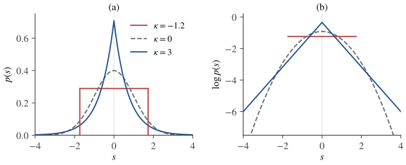
The sign of the kurtosis does not determine the shape of a density, but typical cases look as follows. Super-Gaussian variables usually have heavier tails than a Gaussian of the same variance, and often a sharper peak; kurtosis measures the tails rather than the peak (Westfall, 2014). The standard examples are sparse signals, which are mostly close to zero and occasionally large: speech (Gazor & Zhang, 2003), the outputs of edge filters applied to natural images (Bell & Sejnowski, 1997), and the spatial maps of fMRI networks (Chapter 14第 14 章). Sub-Gaussian variables are usually flatter, with light tails, and often bounded or multimodal: a uniform variable, a sinusoid with random phase, a binary communication symbol. There are exceptions: a variable equal to ±1 with probability 0.49 each and to ±5 with probability 0.01 each is bimodal, yet its normalized kurtosis is +3.15. Figure 2.1图 2.1 compares three typical unit-variance densities.
Figure 2.1. Unit-variance densities with negative, zero and positive kurtosis: uniform (κ=−1.2), Gaussian (κ=0) and Laplace (κ=3). (a) Densities. (b) Log-densities: the Laplace tails decay linearly and the Gaussian tails quadratically, while the uniform density vanishes outside [−3,3].图 2.1 峭度为负、零、正的单位方差密度:均匀分布(κ=−1.2)、高斯分布(κ=0)与拉普拉斯分布(κ=3)。(a)密度。(b)对数密度:拉普拉斯分布的尾部线性衰减,高斯分布的尾部按二次衰减,而均匀分布的密度在 [−3,3] 之外为零。
Proposition 2.11 (properties of kurtosis)命题 2.11(峭度的性质)
Let y, y1 and y2 have finite fourth moments, and let σ2=Var(y)>0.
设 y、y1、y2 的四阶矩有限,σ2=Var(y)>0。
kurt(αy+c)=α4kurt(y) for constants α and c; hence the normalized kurtosis is invariant under affine maps with α=0.
If y1 and y2 are independent, kurt(y1+y2)=kurt(y1)+kurt(y2). Consequently, for independent unit-variance sources, kurt(∑iqisi)=∑iqi4κi.
kurt(y)≥−2σ4, with equality if and only if y takes the two values μ±σ with probability 21 each.
(1) and (2) follow from multilinearity, shift invariance and additivity in Proposition 2.8命题 2.8. (3) By Jensen's inequality for the convex function u↦u2, E[(y−μ)4]=E[((y−μ)2)2]≥(E[(y−μ)2])2=σ4, so kurt(y)≥σ4−3σ4. Since u↦u2 is strictly convex, equality holds if and only if (y−μ)2 is almost surely constant, that is, y=μ±σ; the condition E[y]=μ then forces the two values to have probability 21.
There is no upper bound: the normalized kurtosis of the Student t distribution, 6/(ν−4), grows without limit as ν decreases to 4. Property 2 is the identity behind Chapter 5第 5 章 (Proposition 5.1命题 5.1): a unit-variance mixture ∑iqisi with ∥q∥=1 has a kurtosis that combines the source kurtoses with weights qi4, whose sum ∑iqi4≤(∑iqi2)2=1 equals one only when q has a single nonzero entry. Table 2.1表 2.1 lists the values for common distributions.
Table 2.1. Variance, skewness and normalized kurtosis of common distributions. The unit-variance versions use a=3 (uniform), b=1/2 (Laplace) and λ=1 (exponential).表 2.1 常见分布的方差、偏度与归一化峭度。单位方差的版本取 a=3(均匀分布)、b=1/2(拉普拉斯分布)、λ=1(指数分布)。
Distribution分布
Density or law密度或分布律
Variance方差
Skewness偏度
Normalized kurtosis归一化峭度
uniform on [−a,a][−a,a] 上的均匀分布
2a1on [−a,a](在 [−a,a] 上)
a2/3
0
−6/5
symmetric binary对称二值分布
P(y=±1)=21
1
0
−2
sinusoid, random phase随机相位正弦波
2sinθ, θ uniform on [0,2π)2sinθ,θ 在 [0,2π) 上均匀
1
0
−3/2
Gaussian高斯分布
2πσ1e−y2/(2σ2)
σ2
0
0
Laplace拉普拉斯分布
2b1e−∣y∣/b
2b2
0
3
exponential指数分布
λe−λy, y≥0
1/λ2
2
6
Student t, ν>4Student t,ν>4
∝(1+y2/ν)−(ν+1)/2
ν/(ν−2)
0
6/(ν−4)
The following script draws a million samples from six of these laws, scaled to unit variance, estimates their kurtosis, and then checks the cumulant computation for the rotated uniform pair of Example 2.3例 2.3.
import numpy as np

rng = np.random.default_rng(0)
T = 1_000_000

def kurt(y):                           # fourth cumulant of a sample
    y = y - y.mean()
    return np.mean(y**4) - 3 * np.mean(y**2)**2

def cum22(y1, y2):                     # cum(y1, y1, y2, y2) of a sample
    y1, y2 = y1 - y1.mean(), y2 - y2.mean()
    return (np.mean(y1**2 * y2**2) - np.mean(y1**2) * np.mean(y2**2)
            - 2 * np.mean(y1 * y2)**2)

samples = {                            # unit-variance draws, as in the table
    "uniform":     rng.uniform(-np.sqrt(3), np.sqrt(3), T),
    "laplace":     rng.laplace(0.0, 1 / np.sqrt(2), T),
    "gaussian":    rng.standard_normal(T),
    "binary":      rng.choice([-1.0, 1.0], T),
    "exponential": rng.exponential(1.0, T),
    "student-t10": rng.standard_t(10, T) / np.sqrt(10 / 8),
}
for name, y in samples.items():
    print(f"{name:12s} kurt = {kurt(y):+.3f}")

# two uniform sources rotated by 45 degrees: white but dependent
s1, s2 = rng.uniform(-np.sqrt(3), np.sqrt(3), (2, T))
z1, z2 = (s1 - s2) / np.sqrt(2), (s1 + s2) / np.sqrt(2)
print(f"E[z1 z2]            = {np.mean(z1 * z2):+.3f}")
print(f"cum(z1, z1, z2, z2) = {cum22(z1, z2):+.3f}")
print(f"cum(s1, s1, s2, s2) = {cum22(s1, s2):+.3f}")
The estimated kurtoses are −1.203, +3.002, +0.004, −2.000, +5.881 and +1.016 (the true value for ν=10 is 6/6=1). Only the exponential estimate is visibly off, by about one standard error: the variance of the sample kurtosis involves the eighth moment, and the delta method (Section A.8第 A.8 节) puts the standard error at about 0.11 here. The last three lines print +0.000, −0.602 and +0.000: the rotated pair is uncorrelated but has the predicted cross-cumulant −0.6, and the independent pair has none.
Cumulants summarize a distribution by a few numbers; entropy summarizes it through its whole density. For a discrete variable, Shannon's entropy (Shannon, 1948) measures the average uncertainty of an outcome. Its continuous counterpart is differential entropy (Cover & Thomas, 2006).
Let y∈Rd have density p. Its differential entropy is H(y)=−∫p(u)logp(u)du=−E[logp(y)], whenever the integral exists. For several random vectors, H(y1,…,yk) is the entropy of the stacked vector.
Three examples follow directly from the definition. A uniform density on an interval of length L has H=logL; for the unit-variance uniform law, L=23 and H=log(23)≈1.2425. For N(μ,σ2), −logp(y)=21log(2πσ2)+(y−μ)2/(2σ2), whose expectation gives H=21log(2πeσ2), or 1.4189 at unit variance; in the same way a Gaussian vector with covariance Σ has H=21log((2πe)ddetΣ). For the Laplace density e−∣y∣/b/(2b), −logp(y)=log(2b)+∣y∣/b and E∣y∣=b, so H=1+log(2b), or 1+21log2≈1.3466 at unit variance.
Differential entropy differs from discrete entropy in two ways. It can be negative (the uniform density on [0,21] has entropy −log2), and it depends on scale: H(αy)=H(y)+log∣α∣. Both facts are special cases of the next proposition. The quantities that ICA uses, mutual information and negentropy, are combinations of entropies in which these changes cancel.
Proposition 2.13 (entropy under linear maps)命题 2.13(线性变换下的熵)
Let y∈Rd have a density and finite entropy, let A∈Rd×d be invertible and b∈Rd. Then H(Ay+b)=H(y)+log∣detA∣. More generally, if f is a continuously differentiable bijection of Rd onto an open set whose Jacobian matrix Jf is nonsingular everywhere, then H(f(y))=H(y)+E[log∣detJf(y)∣] whenever the right-hand side is finite.
By the change-of-variables formula, f(y) has the density pf(y)(f(u))=py(u)/∣detJf(u)∣. Hence H(f(y))=−E[logpf(y)(f(y))]=−E[logpy(y)]+E[log∣detJf(y)∣]. For f(u)=Au+b the Jacobian is the constant matrix A.
Two consequences recur in later chapters. Orthogonal transformations preserve entropy, H(Qy)=H(y), because ∣detQ∣=1: rotating whitened data does not change their joint entropy. And for y=Wx with W invertible, H(y)=H(x)+log∣detW∣; this is how the term log∣detW∣ enters the likelihood of ICA in Chapter 6第 6 章.
D(p∥q)≥0, with equality if and only if p=q almost everywhere.
D(p∥q)≥0,等号成立当且仅当 p=q 几乎处处成立。
Proof.证明
We may assume D(p∥q)<∞. Let y∼p. By Jensen's inequality for the concave logarithm, −D(p∥q)=E[log(q(y)/p(y))]≤logE[q(y)/p(y)]=log∫{p>0}q(u)du≤log1=0. Since the logarithm is strictly concave, equality in the first step requires q/p to be constant on {p>0}, and equality in the second requires ∫{p>0}q=1; together they give q=p almost everywhere.
The divergence was introduced by Kullback and Leibler (1951). It is not symmetric, and it is not a metric. It is invariant under reparametrization: if both densities are transformed by the same map f as in Proposition 2.13命题 2.13, the Jacobian factors cancel in the ratio p/q. Its first use here is a classical extremal property of the Gaussian.
Hence H(y)≤21log((2πe)ddetΣ), the entropy of N(μ,Σ), with equality if and only if y is Gaussian.
因此 H(y)≤21log((2πe)ddetΣ),即 N(μ,Σ) 的熵;等号成立当且仅当 y 是高斯的。
Proof.证明
We have −logpG(u)=21log((2π)ddetΣ)+21(u−μ)⊤Σ−1(u−μ). Its expectation under p depends only on the mean and covariance of y: since E[(y−μ)⊤Σ−1(y−μ)]=tr(Σ−1Σ)=d, it equals 21log((2πe)ddetΣ), the same value as for a Gaussian y. Therefore D(p∥pG)=−H(y)+E[−logpG(y)]=21log((2πe)ddetΣ)−H(y), which is nonnegative by Lemma 2.15引理 2.15 and zero only when p=pG almost everywhere.
我们有 −logpG(u)=21log((2π)ddetΣ)+21(u−μ)⊤Σ−1(u−μ)。它在 p 下的期望只依赖于 y 的均值与协方差:由于 E[(y−μ)⊤Σ−1(y−μ)]=tr(Σ−1Σ)=d,这个期望等于 21log((2πe)ddetΣ),与 y 为高斯时的值相同。因此 D(p∥pG)=−H(y)+E[−logpG(y)]=21log((2πe)ddetΣ)−H(y);由Lemma 2.15引理 2.15,它非负,且仅当 p=pG 几乎处处成立时为零。
Among all distributions with a given covariance, the Gaussian is the most disordered. This is the information-theoretic side of the intuition in Section 1.5第 1.5 节: mixing independent signals makes them more Gaussian, so a measure of distance from the Gaussian can guide separation.
Let y=(y1,…,yk) have joint density py and marginal densities pyi. The mutual information of y1,…,yk is the divergence of the joint density from the product of its marginals,
Proposition 2.18 (properties of mutual information)命题 2.18(互信息的性质)
(a) I(y)≥0, with equality if and only if the components of y are independent. (b) If f1,…,fn are continuously differentiable bijections of R onto open intervals with nonvanishing derivatives, then I(f1(y1),…,fn(yn))=I(y1,…,yn). In particular, mutual information does not change when the components are rescaled, change sign or are permuted.
(a)I(y)≥0,等号成立当且仅当 y 的各分量独立。(b)若 f1,…,fn 都是从 R 到某个开区间的连续可微双射,且导数处处不为零,则 I(f1(y1),…,fn(yn))=I(y1,…,yn)。特别地,对各分量作缩放、改变符号或重新排列,互信息都不变。
Proof.证明
(a) follows from Lemma 2.15引理 2.15 and statement 3 of Proposition 2.2命题 2.2. (b) Assume the entropies are finite. The Jacobian of u↦(f1(u1),…,fn(un)) is diagonal, so by Proposition 2.13命题 2.13 the joint entropy changes by ∑iE[log∣fi′(yi)∣], while each marginal entropy H(fi(yi)) changes by E[log∣fi′(yi)∣]. The changes cancel in ∑iH(yi)−H(y), and a permutation only reorders the sum. (Without finite entropies, use the invariance of the divergence under reparametrization.)
the starting point of Chapter 6第 6 章 ((6.4)). The entropy H(x) does not depend on W, so minimizing the mutual information of the outputs involves only the marginal entropies and log∣detW∣.
Let y∈Rd have a density, finite entropy and nonsingular covariance Σ, and let yG be a Gaussian vector with the same mean and covariance. The negentropy of y is J(y)=H(yG)−H(y)=21log((2πe)ddetΣ)−H(y). For a scalar, J(y)=21log(2πeVar(y))−H(y).
Proposition 2.20 (properties of negentropy)命题 2.20(负熵的性质)
(a) J(y)≥0, with equality if and only if y is Gaussian. (b) J(y)=D(py∥pG), where pG is the Gaussian density with the same mean and covariance. (c) J(Ay+b)=J(y) for every invertible A and every b.
(a)J(y)≥0,等号成立当且仅当 y 是高斯的。(b)J(y)=D(py∥pG),其中 pG 是均值、协方差与 y 相同的高斯密度。(c)对任意可逆的 A 与任意 b,J(Ay+b)=J(y)。
Proof.证明
(a) and (b) restate Proposition 2.16命题 2.16. (c) The vector Ay+b has covariance AΣA⊤, and the Gaussian vector with its mean and covariance is AyG+b. By Proposition 2.13命题 2.13, H(Ay+b) and H(AyG+b) both exceed the original entropies by log∣detA∣, so their difference is unchanged.
Negentropy is the information-theoretic measure of non-Gaussianity: unlike entropy it does not depend on scale, and unlike kurtosis it uses the whole density. From the entropies of Section 2.6第 2.6 节, J=21log(πe/6)≈0.1765 for the uniform law and J=21log(πe)−1≈0.0724 for the Laplace law, whatever the variance. The two measures need not agree: the Laplace law has the larger absolute kurtosis (3 against 1.2) but the smaller negentropy.
The two information measures are linked. For any y with nonsingular covariance C,
这两个信息论量之间有联系。对任何协方差 C 非奇异的 y,
I(y)=J(y)−i=1∑nJ(yi)+21logdetC∏i=1nCii(2.5)
(Exercise 2.6习题 2.6). If y=Uz with z white and U orthogonal, the last term vanishes and J(y)=J(z) does not depend on U, so minimizing the mutual information of the outputs is the same as maximizing the sum of their negentropies. Chapter 6第 6 章 develops this equivalence (Proposition 6.4命题 6.4), connects it with maximum likelihood, and replaces negentropy, which requires a density, by approximations that can be estimated from samples (Section 6.7第 6.7 节).
Independence means that the joint distribution factorizes; equivalently, E[g(y1)h(y2)]=E[g(y1)]E[h(y2)] for all bounded g and h, or the characteristic function factorizes. Uncorrelatedness is the linear special case and is much weaker, except for jointly Gaussian vectors.
Cumulants are the Taylor coefficients of the logarithm of the characteristic function. They are symmetric and multilinear, add up over independent summands, vanish when their arguments split into independent groups, and vanish beyond order two for Gaussian variables.
For x=As with independent sources, cum(xi,xj,xk,xl)=∑paipajpakpalpκp: fourth-order statistics see the individual columns of A, which the covariance cannot.
Kurtosis, kurt(y)=E[y4]−3(E[y2])2 for zero-mean y, is the fourth cumulant. Its sign separates sub-Gaussian from super-Gaussian variables, and the normalized kurtosis is at least −2.
Differential entropy changes by log∣detA∣ under y↦Ay, and at fixed covariance it is largest for the Gaussian.
Mutual information I(y)=∑iH(yi)−H(y)≥0 vanishes exactly when the components are independent; negentropy J≥0 vanishes exactly for Gaussian vectors and is invariant under invertible linear maps.
独立意味着联合分布可以分解;等价地,对一切有界的 g 与 h 有 E[g(y1)h(y2)]=E[g(y1)]E[h(y2)],或者特征函数可以分解。不相关只是其中的线性特例,要弱得多;联合高斯向量是例外。
累积量是特征函数对数的 Taylor 系数。它们对称、多重线性,对独立的加项可加;当自变量能分成相互独立的两组时为零;对高斯变量,二阶以上的累积量全为零。
对源独立的 x=As,cum(xi,xj,xk,xl)=∑paipajpakpalpκp:四阶统计量能看到 A 的每一列,而协方差做不到。
Compute the normalized kurtosis of the uniform distribution on [−a,a] and of the sinusoid y=2sinθ with θ uniform on [0,2π), and check the entries of Table 2.1表 2.1.
Uniform: E[y2]=2a1∫−aau2du=a2/3 and E[y4]=a4/5, so kurt(y)=a4/5−3a4/9=−2a4/15, and dividing by (a2/3)2=a4/9 gives −18/15=−6/5. Sinusoid: E[sin2θ]=21, so E[y2]=1; since sin4θ=(3−4cos2θ+cos4θ)/8, E[sin4θ]=3/8 and E[y4]=4⋅3/8=3/2. Hence kurt(y)=3/2−3=−3/2. Both laws are symmetric, so their skewness is zero.
Let x∼N(0,1), let ε be independent of x with P(ε=1)=P(ε=−1)=21, and set y=εx. Show that y∼N(0,1) and Cov(x,y)=0, but that x and y are dependent. Why does this not contradict Proposition 2.6命题 2.6?
设 x∼N(0,1),ε 与 x 独立且 P(ε=1)=P(ε=−1)=21,令 y=εx。证明 y∼N(0,1) 且 Cov(x,y)=0,但 x 与 y 不独立。为什么这与Proposition 2.6命题 2.6不矛盾?
Show solution查看解答
By symmetry of x, P(y≤u)=21P(x≤u)+21P(−x≤u)=P(x≤u), so y∼N(0,1). Also Cov(x,y)=E[εx2]=E[ε]E[x2]=0. But ∣y∣=∣x∣, so P(∣x∣≤1,∣y∣≤1)=P(∣x∣≤1)≈0.683, while P(∣x∣≤1)P(∣y∣≤1)≈0.6832≈0.466: the variables are dependent. There is no contradiction because (x,y) is not jointly Gaussian: x+y=(1+ε)x equals 0 with probability 21 and is otherwise distributed as 2x, which is neither Gaussian nor constant.
Let y be exponential with rate λ. Using φy(ω)=λ/(λ−iω), show that κj(y)=(j−1)!/λj for all j≥1. Deduce that the skewness is 2 and the normalized kurtosis is 6 for every λ, and check κ3 and κ4 against the raw-moment formulas of Section 2.4第 2.4 节, using E[yj]=j!/λj.
For ∣ω∣<λ, logφy(ω)=−log(1−iω/λ)=∑j≥1j1(λiω)j=∑j≥1λj(j−1)!j!(iω)j, so κj=(j−1)!/λj. Then Var(y)=κ2=1/λ2, the skewness is κ3/κ23/2=(2/λ3)λ3=2, and the normalized kurtosis is κ4/κ22=(6/λ4)λ4=6. With λ=1 the raw moments are mj=j!, and the formulas give κ3=6−3⋅2⋅1+2=2 and κ4=24−4⋅6−3⋅4+12⋅2−6=6, as they should; other values of λ only rescale y.
Derive the negentropies J=21log(πe/6) of the uniform law and J=21log(πe)−1 of the Laplace law, and explain why they do not depend on the variance. Which of the two laws is “more non-Gaussian” according to kurtosis, and which according to negentropy?
By Proposition 2.20命题 2.20(c), J(αy)=J(y), so we may take unit variance. Uniform on [−3,3]: H=log(23)=21log12, so J=21log(2πe)−21log12=21log(πe/6)≈0.1765. Laplace with b=1/2: H=1+log(2b)=1+21log2, so J=21log(2πe)−1−21log2=21log(πe)−1≈0.0724. By absolute normalized kurtosis the Laplace law is further from the Gaussian (3 against 1.2); by negentropy the uniform law is (0.1765 against 0.0724). Kurtosis is dominated by the tails, negentropy weighs the whole density, and the bounded support of the uniform law makes its density very different from a Gaussian one.
Derive (2.2) from Definition 2.7定义 2.7: for zero-mean x1,…,x4 with finite fourth moments, expand logφx(ω) to fourth order and identify the coefficient of ω1ω2ω3ω4. Then use the formula to check directly that cum(y1,y1,y2,y2)=0 when y1 and y2 are independent with zero mean.
Let cab=E[xaxb], mabc=E[xaxbxc] and mabcd=E[xaxbxcxd]. Expanding the exponential to fourth order (no first-order term, because the means vanish), φx(ω)=1+u with
Then log(1+u)=u−u2/2+O(∣u∣3), where u3=O(∥ω∥6) and, up to o(∥ω∥4), u2=41S2 with S=∑a,bcabωaωb. Since cum(x1,x2,x3,x4) is the fourth mixed derivative at 0 (the factor (−i)4 equals 1), it is the coefficient of ω1ω2ω3ω4 in this expansion. In u, the 24 orderings of (1,2,3,4) in the quartic sum contribute 241⋅24m1234=m1234. In S2, the monomial ω1ω2ω3ω4 arises from products of two terms of S whose index pairs split {1,2,3,4}; there are three such splits, each term of S with a=b appears twice (cab=cba), and the two factors can be taken in either order, so the coefficient is 8(c12c34+c13c24+c14c23). With the factor −21⋅41, the coefficient in logφx is m1234−c12c34−c13c24−c14c23, which is (2.2). For independent zero-mean y1 and y2, the formula gives cum(y1,y1,y2,y2)=E[y12y22]−E[y12]E[y22]−2(E[y1y2])2=E[y12]E[y22]−E[y12]E[y22]−0=0.
Prove (2.5). Deduce that if z is white and y=Uz with U orthogonal, then I(y)=J(z)−∑iJ(yi), and that the separating rotations are exactly the maximizers of ∑iJ(yi) whenever z=A~s with A~ orthogonal and independent sources, at most one of them Gaussian.
证明 (2.5)。由此推出:若 z 是白的,y=Uz 且 U 正交,则 I(y)=J(z)−∑iJ(yi);并且当 z=A~s(A~ 正交,源独立且至多一个是高斯的)时,使 ∑iJ(yi) 最大的旋转恰好就是能实现分离的旋转。
Show solution查看解答
By the definition of negentropy, H(yi)=21log(2πeCii)−J(yi) and H(y)=21log((2πe)ndetC)−J(y). Substituting into I(y)=∑iH(yi)−H(y), the terms 21log(2πe) cancel (n of them on each side) and we obtain I(y)=J(y)−∑iJ(yi)+21(∑ilogCii−logdetC), which is (2.5). If y=Uz with z white, then C=UIU⊤=I, so the last term is 21log(1/1)=0, and J(y)=J(z) by Proposition 2.20命题 2.20(c). Hence I(y)=J(z)−∑iJ(yi), where J(z) does not depend on U. Since I(y)≥0 with equality exactly for independent outputs (Proposition 2.18命题 2.18), ∑iJ(yi)≤J(z) for every U, with equality exactly when the outputs are independent. A separating rotation, UA~=ΠD, makes them independent and therefore attains the maximum. Conversely, any maximizer has independent outputs, and when at most one source is Gaussian, Comon's theorem (Theorem 4.6定理 4.6) shows that it separates.
由负熵的定义,H(yi)=21log(2πeCii)−J(yi),H(y)=21log((2πe)ndetC)−J(y)。代入 I(y)=∑iH(yi)−H(y),两边各 n 个 21log(2πe) 相互抵消,得到 I(y)=J(y)−∑iJ(yi)+21(∑ilogCii−logdetC),即 (2.5)。若 y=Uz 且 z 是白的,则 C=UIU⊤=I,最后一项为 21log(1/1)=0;又由Proposition 2.20命题 2.20(c),J(y)=J(z)。因此 I(y)=J(z)−∑iJ(yi),其中 J(z) 与 U 无关。由于 I(y)≥0,且仅当输出独立时取等号(Proposition 2.18命题 2.18),对每个 U 都有 ∑iJ(yi)≤J(z),等号恰在输出独立时成立。能实现分离的旋转(UA~=ΠD)使输出独立,因而达到最大值。反之,任何最大值点都使输出独立;当至多一个源是高斯的时,Comon 定理(Theorem 4.6定理 4.6)表明它能实现分离。