Part IV · Chapter 11第四部分 · 第 11 章
Noise, Model Order and Reliability噪声、模型阶数与可靠性
Noisy ICA, PCA reduction and model-order selection, split and unstable components, and how to assess the reliability of an ICA decomposition.
含噪 ICA、PCA 降维与模型阶数选择、分裂与不稳定的成分,以及如何评估一次 ICA 分解的可靠性。
11.1 Beyond the noiseless square model超越无噪声的方阵模型
The theory of the previous chapters assumes that holds exactly and that the number of sources is known. Real recordings violate this in three ways that matter. Sensors add noise, so the data follow . The number of sources is unknown and usually much smaller than the number of sensors: a 64-channel EEG recording or an fMRI data set with hundreds of time points is reduced to a few dozen components, and someone has to decide how many. Finally, ICA algorithms are iterative and randomly initialized and their contrasts have several local optima, so two runs on the same data can return different components.
前面各章的理论假设 严格成立,而且源的个数已知。真实数据在三个要紧的方面违背这些假设。传感器会引入噪声,所以数据服从 。源的个数未知,而且通常远小于传感器个数:一份 64 导联的 EEG 记录,或一份有几百个时间点的 fMRI 数据,往往被降到几十个成分,而降到多少需要有人决定。最后,ICA 算法是迭代的、随机初始化的,其对比函数有多个局部最优,所以在同一份数据上运行两次,可能得到不同的成分。
This chapter takes up the three questions in turn: what noise does to ICA (Section 11.2第 11.2 节), how to choose the number of components and what happens when it is wrong (Section 11.3第 11.3 节 and Section 11.4第 11.4 节), and how to judge whether an estimated component can be trusted (Section 11.5第 11.5 节 and Section 11.6第 11.6 节).
本章依次讨论这三个问题:噪声对 ICA 有什么影响(Section 11.2第 11.2 节);如何选择成分个数,以及选错了会怎样(Section 11.3第 11.3 节与Section 11.4第 11.4 节);如何判断一个估计出的成分是否可信(Section 11.5第 11.5 节与Section 11.6第 11.6 节)。
11.2 Noisy ICA含噪 ICA
The noisy model is
含噪模型为
with of full column rank (), sources as in Assumption 1.1假设 1.1 with unit variance, and noise independent of the sources. Isotropic noise is the standard assumption; noise with a known covariance is reduced to it by replacing with . The covariance of the data is . If are the nonzero eigenvalues of , the eigenvalues of are
其中 列满秩(),源满足Assumption 1.1假设 1.1且方差为一,噪声与源独立。各向同性噪声是标准假设;若噪声协方差 已知,用 代替 即可化为这种情形。数据的协方差为 。若 是 的非零特征值,则 的特征值为
and the leading eigenvectors span the column space of . This is why PCA reduction (Section 3.6第 3.6 节) keeps the signal, and it is the starting point of order selection. Four consequences of noise follow.
并且前 个特征向量张成 的列空间。这就是 PCA 降维(Section 3.6第 3.6 节)能保留信号的原因,也是选择阶数的出发点。噪声带来以下四个后果。
Whitening is biased白化有偏
Proposition 11.1 (whitening noisy data)命题 11.1(含噪数据的白化)
Let hold the leading eigenvectors of and , and let with orthogonal (for this is every whitening matrix). Then
设 由 的前 个特征向量组成,,并设 ,其中 为正交矩阵( 时这就是全部白化矩阵)。则
so the singular values of are , , and is not orthogonal when . The bias-corrected matrix makes orthogonal.
因此 的奇异值为 (),当 时 不是正交矩阵。经偏差校正的矩阵 则使 成为正交矩阵。
Proof.证明
Since has its column space spanned by , . Hence , and has eigenvalues . Replacing by gives .
由于 的列空间由 张成,有 。因此 ,而 的特征值为 。把 换成 就得到 。
After ordinary whitening, an algorithm that searches over rotations therefore cannot, in general, reach a separating matrix. A rotation can turn into a scaled permutation matrix only if the columns of are orthogonal; since , this happens exactly when the columns of are orthogonal. The distortion is of relative size and is largest along the weakest signal direction. Bias correction requires , which can be estimated from the discarded eigenvalues when (see probabilistic PCA below). Unlike the noiseless case, equivariance is also lost: the outputs contain a noise term that depends on and hence on .
因此,在普通白化之后,在旋转中搜索的算法一般无法到达分离矩阵。只有当 的各列相互正交时,旋转才能把它变成带尺度的置换矩阵;而 ,所以这恰好发生在 的各列相互正交的时候。畸变的相对大小为 ,沿最弱的信号方向最大。偏差校正需要知道 ;当 时,可以由被舍弃的特征值估计它(见下文的概率 PCA)。与无噪声情形不同,等变性也不再成立:输出 含有依赖于 、从而依赖于 的噪声项。
Higher-order cumulants ignore Gaussian noise高阶累积量对高斯噪声“视而不见”
Cumulants are additive for independent summands and vanish beyond order two for Gaussian variables (Proposition 2.8命题 2.8). Hence the fourth-order cumulants of noisy data are those of the noiseless mixture,
独立随机变量之和的累积量等于各自累积量之和,而高斯变量二阶以上的累积量全为零(Proposition 2.8命题 2.8)。因此含噪数据的四阶累积量与无噪声混合的完全相同:
After bias-corrected whitening , a unit vector gives with a unit vector, exactly as without noise; so the source directions remain the maxima of on the sphere (Theorem 5.3定理 5.3), and cumulant methods such as JADE remain consistent once the whitening is corrected. Contrasts built from other nonlinearities, such as or a likelihood, are biased by noise. Hyvärinen (1999) introduced “Gaussian moments”, expectations of Gaussian functions of the output whose noise bias can be removed in closed form, together with a modified FastICA.
经偏差校正的白化 之后,对单位向量 有 ,其中 也是单位向量,与无噪声时完全一样;所以源方向仍然是 在球面上的极大点(Theorem 5.3定理 5.3),白化一经校正,JADE 这类累积量方法仍然相合。基于其他非线性函数(如 或似然)的对比函数则会被噪声带偏。Hyvärinen(1999)提出了“高斯矩”,即输出的高斯函数的期望,其噪声偏差可以用闭式去除,并给出了相应修改的 FastICA。
The sources cannot be recovered exactly源无法精确恢复
Even with known, noise cannot be removed. For the unmixed outputs carry noise with covariance , which is large when is ill-conditioned. The linear estimator with the smallest mean squared error is , which accepts a bias (shrinkage toward zero) in exchange for less noise; nonlinear estimators that use the non-Gaussian source densities do better still (Hyvärinen, Karhunen & Oja, 2001). Noisy ICA thus splits into two tasks: estimating , which can be done consistently, and estimating , which can only be done approximately.
即使 已知,噪声也无法去除。 时,解混输出 所含噪声的协方差为 , 病态时它很大。均方误差最小的线性估计量是 ,它以一定的偏差(向零收缩)换取较小的噪声;利用非高斯源密度的非线性估计量还能做得更好(Hyvärinen, Karhunen & Oja, 2001)。因此含噪 ICA 分为两个任务:估计 ,这可以相合地做到;估计 ,这只能近似地做到。
Probabilistic PCA概率 PCA
Probabilistic PCA (Tipping & Bishop, 1999) is the model with Gaussian factors and . Let be the eigenvalues of the sample covariance, the corresponding leading eigenvectors and . The maximum-likelihood estimates are
概率 PCA(Tipping & Bishop, 1999)是模型 ,其中 个因子 为高斯分布,。设 为样本协方差的特征值, 为相应的前 个特征向量,。最大似然估计为
where is an arbitrary orthogonal matrix. The noise variance is the average of the discarded eigenvalues, and the factor loadings are determined only up to the rotation , because Gaussian factors can be rotated freely. That rotation is exactly what ICA determines when the factors are non-Gaussian. A noisy-ICA pipeline therefore estimates the signal subspace and by probabilistic PCA, whitens with the bias-corrected matrix , and finds the rotation by ICA; probabilistic ICA for fMRI (Beckmann & Smith, 2004) follows this route (Chapter 14第 14 章).
其中 是任意正交矩阵。噪声方差就是被舍弃特征值的平均;因子载荷只能确定到旋转 ,因为高斯因子可以自由旋转。而当因子非高斯时,这个旋转恰好由 ICA 确定。因此含噪 ICA 的流程是:用概率 PCA 估计信号子空间和 ,用经偏差校正的矩阵 白化,再用 ICA 求出旋转。fMRI 中的概率 ICA(Beckmann & Smith, 2004)走的就是这条路(Chapter 14第 14 章)。
11.3 Choosing the number of components选择成分个数
When , ICA is run on the -dimensional principal subspace, and , the model order, must be chosen. In the population, (11.2) shows eigenvalues above a flat floor . In a sample the noise eigenvalues spread around , the more so the larger , and a weak signal eigenvalue can disappear among them. A principled choice compares, for each candidate , how well the “ signals plus white noise” covariance fits the data against how many parameters it uses.
当 时,ICA 在 维主子空间上运行,而 ,即模型阶数,必须选定。在总体层面,(11.2) 显示有 个特征值高出平坦的噪声底 。在样本中,噪声特征值会在 周围散开, 越大散得越开,较弱的信号特征值可能淹没其中。有原则的选择方法是:对每个候选的 ,权衡“ 个信号加白噪声”这一协方差模型对数据的拟合程度与它所用的参数个数。
The maximum-likelihood fit of that model is the probabilistic PCA solution, and its maximized Gaussian log-likelihood depends on the eigenvalues only through the ratio of the geometric to the arithmetic mean of the smallest ones (Exercise 11.5习题 11.5):
这个模型的最大似然拟合就是概率 PCA 的解,其最大化后的高斯对数似然只通过最小的 个特征值的几何平均与算术平均之比依赖于特征值(Exercise 11.5习题 11.5):
Here is the maximized likelihood of the model with signals and that of an unrestricted covariance, which does not depend on . The logarithm on the right is at most zero and vanishes only when the smallest eigenvalues are equal. The model has free parameters ( signal eigenvalues, , and orthonormal eigenvectors in ). The order is chosen by minimizing
其中 是含 个信号的模型的最大似然值, 是协方差不受限制时的最大似然值,后者与 无关。右边的对数不大于零,且仅当最小的 个特征值全部相等时为零。该模型有 个自由参数( 个信号特征值、,以及 中的 个标准正交特征向量)。阶数通过最小化下列准则来选择:
the criteria of Akaike (1974) and of Rissanen (1978), written relative to , which shifts them by a constant and does not change the minimizer; MDL coincides with half the Bayesian information criterion of Schwarz (1978). Wax and Kailath (1985) derived these eigenvalue forms for complex-valued array data, where the likelihood term carries instead of and the parameter count is ; the forms above are the real-valued analogues. Because its penalty grows with , MDL is consistent for i.i.d. Gaussian data, whereas AIC tends to overestimate the order (Wax & Kailath, 1985). Minka (2000) proposed a Bayesian alternative, a Laplace approximation to the evidence of the probabilistic PCA model, which outperformed cross-validation and other methods in his simulations; it is used in probabilistic ICA (Beckmann & Smith, 2004).
这分别是 Akaike(1974)和 Rissanen(1978)的准则,这里写成相对于 的形式,只差一个常数,不改变最小点;MDL 恰为 Schwarz(1978)的贝叶斯信息准则的一半。Wax 和 Kailath(1985)针对复值阵列数据推导了这些基于特征值的形式,那里似然项中是 而不是 ,参数个数为 ;上面的形式是相应的实值版本。由于 MDL 的惩罚项随 增长,它对独立同分布的高斯数据是相合的,而 AIC 往往高估阶数(Wax & Kailath, 1985)。Minka(2000)提出了一个贝叶斯替代方案:用 Laplace 近似计算概率 PCA 模型的证据(evidence),在他的模拟中优于交叉验证和其他方法;概率 ICA 采用了这一方法(Beckmann & Smith, 2004)。
Dependent samples相依样本
All of these criteria treat the samples as independent. Temporally or spatially correlated samples carry less information than their number suggests: the sample covariance fluctuates more, the noise eigenvalues spread more, and the criteria read the spread as signal and overestimate the order. Li, Adalı and Calhoun (2007) proposed to subsample the data so that the retained samples are effectively independent, choosing the subsampling depth from an entropy-rate measure of the dependence, and to apply the criteria to the subsampled data. In the GIFT toolbox, which implements this method, the eigenvalues of the subsampled data are further divided by the corresponding quantiles of the Marčenko–Pastur law (Section 3.6第 3.6 节) for the effective sample size, and the order is taken at the first local minimum of MDL rather than at its global minimum. The script below shows the effect with Laplace sources in sensors, where sources and noise are either white or first-order autoregressive with coefficient .
上述准则都把 个样本当作相互独立。时间上或空间上相关的样本所含的信息比其个数所暗示的要少:样本协方差波动更大,噪声特征值散得更开,而准则会把这种散开误读为信号,从而高估阶数。Li、Adalı 和 Calhoun(2007)提出对数据降采样,使保留下来的样本近似独立(降采样的间隔由衡量相依程度的熵率指标确定),再对降采样后的数据应用这些准则。在实现了这一方法的 GIFT 工具箱中,降采样数据的特征值还要再除以按有效样本量计算的 Marčenko–Pastur 分布(Section 3.6第 3.6 节)的相应分位数,阶数取 MDL 的第一个局部极小点,而不是全局极小点。下面的脚本用 个传感器中的 个拉普拉斯源演示这一效应,源和噪声或者是白的,或者是系数 的一阶自回归过程。
import numpy as np

def order_criteria(X):
    """Orders chosen by AIC and MDL from the sample covariance eigenvalues."""
    m, T = X.shape
    ell = np.sort(np.linalg.eigvalsh(np.cov(X)))[::-1]
    aic, mdl = [], []
    for k in range(m):
        tail = ell[k:]                      # the m - k smallest eigenvalues
        loglr = (m - k) * (np.mean(np.log(tail)) - np.log(np.mean(tail)))
        p = m * k - k * (k - 1) / 2 + 1     # free parameters of the model
        aic.append(-T * loglr + 2 * p)
        mdl.append(-T / 2 * loglr + p / 2 * np.log(T))
    return int(np.argmin(aic)), int(np.argmin(mdl))

def ar1(E, phi):
    """Turn each row of white noise E into a unit-variance AR(1) series."""
    Y = np.empty_like(E)
    Y[:, 0] = E[:, 0]
    for t in range(1, E.shape[1]):
        Y[:, t] = phi * Y[:, t - 1] + np.sqrt(1 - phi ** 2) * E[:, t]
    return Y

rng = np.random.default_rng(1)
m, n, T = 30, 8, 5000
A = rng.normal(size=(m, n))
S = rng.laplace(0, 1 / np.sqrt(2), (n, T))
N = rng.normal(size=(m, T))
for phi in [0.0, 0.9]:
    X = A @ ar1(S, phi) + ar1(N, phi)
    print(f"phi = {phi}: all samples (AIC, MDL) = {order_criteria(X)}, "
          f"every 10th sample = {order_criteria(X[:, ::10])}")
The script prints
脚本输出
phi = 0.0: all samples (AIC, MDL) = (9, 8), every 10th sample = (8, 8)
phi = 0.9: all samples (AIC, MDL) = (29, 18), every 10th sample = (9, 8)
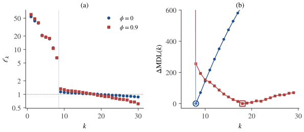
With independent samples MDL finds the eight sources and AIC overestimates by one. With dependent samples both fail, AIC choosing the largest admissible order. Keeping every tenth sample restores the behaviour seen with independent samples (MDL 8, AIC 9), although it discards 90% of the data; ten is close to the factor by which the dependence inflates the variance of a sample covariance between two such AR(1) series. Figure 11.1图 11.1 shows why: the noise eigenvalues of the dependent data form a tilted floor rather than a flat one, and MDL reaches its minimum far beyond .
样本独立时,MDL 找到了全部八个源,AIC 多估了一个。样本相依时两者都失败了,AIC 甚至选了允许的最大阶数。每十个样本保留一个,尽管丢掉了 90% 的数据,却恢复了独立样本时的结果(MDL 为 8,AIC 为 9);10 接近于这种相依性使两个 AR(1) 序列之间样本协方差的方差放大的倍数 。Figure 11.1图 11.1说明了原因:相依数据的噪声特征值构成倾斜的而不是平坦的“底”,MDL 的最小值远在 之后。
11.4 Too few or too many components: merged and split components成分过少或过多:合并与分裂
A wrong order has characteristic consequences. If , PCA keeps the directions of largest variance and discards directions that still contain signal; the sources that live partly in the discarded directions cannot be separated and appear as merged components, mixtures of two or more sources. The typical victims are sources with nearly collinear mixing columns. Their sum direction has large variance and their difference direction small variance, proportional to for columns of equal norm at angle (Exercise 11.3习题 11.3), so the difference is the first thing to be discarded. In fMRI terms, two regions with similar time courses are found as one network.
阶数选错会带来典型的后果。若 ,PCA 只保留方差最大的 个方向,丢掉了仍含信号的方向;部分落在被丢弃方向上的那些源无法分开,表现为合并的成分,即两个或更多源的混合。最典型的受害者是混合列几乎共线的源:它们的和方向方差大,差方向方差小,对夹角为 、范数相等的两列,后者与 成正比(Exercise 11.3习题 11.3),所以差方向最先被丢掉。用 fMRI 的话说,时间过程相近的两个脑区会被当成一个网络。
If , the extra dimensions contain mostly noise. With Gaussian noise and enough samples, ICA leaves the sources intact and returns nearly Gaussian components, which are harmless once recognized. Two problems remain. First, components that are merged at a lower order may split at a higher one, and whether the parts are distinct sources or fragments of one process is a question about the data that ICA cannot answer. Second, when is large relative to , ICA overfits: with too few samples per dimension it returns components concentrated on a single spike or bump, whose apparent non-Gaussianity is created by the fit itself (Särelä & Vigário, 2003). Overfitting is a reason to reduce the dimension before ICA even when the data contain many genuine sources. In practice the cost of overestimation is not negligible: on fMRI data, Li, Adalı and Calhoun (2007) found that at overestimated orders the estimated components become less stable and task-related activations are estimated less accurately.
若 ,多出来的维度主要是噪声。在高斯噪声且样本充足时,ICA 不会破坏源,只是多返回 个近似高斯的成分,认出来就无害。但仍有两个问题。其一,低阶时被合并的成分在高阶时可能分裂,而分出来的部分是不同的源还是同一过程的碎片,是关于数据的问题,ICA 回答不了。其二,当 相对于 很大时,ICA 会过拟合:每个维度的样本太少,它会返回集中在单个尖峰或鼓包上的成分,其表面上的非高斯性是拟合本身造出来的(Särelä & Vigário, 2003)。即使数据中确实有很多源,这也是在 ICA 之前先降维的一个理由。实践中高估阶数的代价并不可忽略:Li、Adalı 和 Calhoun(2007)在 fMRI 数据上发现,阶数高估时估计出的成分变得不那么稳定,任务相关激活的估计也变差。
Example 11.2 (merging and splitting)例 11.2(合并与分裂)
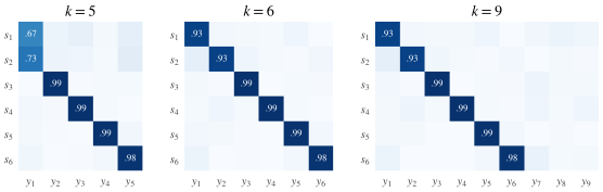
Six unit-variance Laplace sources are mixed into sensors with white noise of standard deviation (), and the column is placed at from . The sample eigenvalues are , followed by a floor near (), and MDL selects . Figure 11.2图 11.2 shows the absolute correlations between the sources and the components found by symmetric FastICA after PCA reduction to . At , and appear together in one component, with correlations and , close to the value of an equal mixture. At they separate, each with correlation , the remainder being noise. At the six sources are unchanged and the three extra components correlate with no source (all absolute correlations below ).
把六个单位方差的拉普拉斯源混合到 个传感器上,加上标准差为 的白噪声(),并让列 与 成 夹角。样本特征值为 ,之后是 附近的噪声底(),MDL 选出 。Figure 11.2图 11.2给出了源与对称 FastICA 所得成分之间的相关系数绝对值,PCA 分别降到 维。 时, 与 一起出现在同一个成分中,相关系数为 和 ,接近等权混合的理论值 。 时它们分开了,相关系数都是 ,余下的是噪声。 时六个源不受影响,另外三个成分与任何源都不相关(相关系数绝对值都低于 )。
There is therefore no single correct order for a real data set: the order sets the scale at which the data are described. A sound practice is to run ICA at several orders, track how components merge and split between them (for example by correlating components across orders), and report the order and how it was chosen. Chapter 14第 14 章 discusses the consequences for brain networks.
因此,对一份真实数据并不存在唯一正确的阶数:阶数决定了描述数据的尺度。稳妥的做法是在几个阶数下分别运行 ICA,追踪成分在阶数之间如何合并与分裂(例如计算不同阶数下成分之间的相关),并报告所用的阶数及其选择方法。Chapter 14第 14 章讨论这对脑网络研究意味着什么。
11.5 Reliability across runs: ICASSO and RAICAR多次运行的可靠性:ICASSO 与 RAICAR
An ICA estimate depends on more than the model. The starting point decides which local optimum the algorithm reaches, and the finite sample perturbs every optimum (Chapter 10第 10 章). A component that appears in every run is more trustworthy than one that appears once. ICASSO (Himberg, Hyvärinen & Esposito, 2004) turns this observation into a procedure.
ICA 的估计结果不只取决于模型。起点决定了算法到达哪个局部最优,有限样本又会扰动每个最优点(Chapter 10第 10 章)。每次运行都出现的成分,比只出现一次的成分更可信。ICASSO(Himberg, Hyvärinen & Esposito, 2004)把这一观察变成了一套流程。
Algorithm 11.3 (ICASSO)算法 11.3(ICASSO)
- Run ICA times, each with a new random initialization and, optionally, on a bootstrap resample of the data (columns of drawn with replacement). Collect all estimated components, in total.
- For every pair of estimates compute the similarity , the absolute correlation between the two estimated components (rows of : time series in temporal ICA, spatial maps in spatial ICA); with unmixing vectors it equals .
- Cluster the estimates by agglomerative hierarchical clustering with average linkage on the dissimilarity , and cut the tree into clusters.
- For each cluster compute the quality index (11.8) and choose as its representative (the centrotype) the estimate with the largest total similarity to the other members of .
- Report the centrotypes ranked by ; compact and isolated clusters ( near 1) indicate reliable components.
- 运行 ICA 次,每次使用新的随机初始化,也可以在数据的自助重抽样样本(有放回地抽取 的列)上运行。收集全部估计成分,共 个。
- 对每一对估计 计算相似度 ,即两个估计成分( 的行:时间 ICA 中是时间序列,空间 ICA 中是空间图)之间相关系数的绝对值;若解混向量为 ,它等于 。
- 以 为相异度,用平均连接的凝聚式层次聚类对这些估计聚类,并把聚类树切成 个簇。
- 对每个簇 计算质量指标 (11.8),并选出与簇内其他成员总相似度最大的估计作为代表(称为中心型,centrotype)。
- 按 排序报告各中心型;紧凑且孤立的簇( 接近 1)表示可靠的成分。
The quality index of a cluster with complement is the average similarity inside the cluster minus the average similarity to the estimates outside it:
簇 (其补集为 )的质量指标,是簇内的平均相似度减去它与簇外估计的平均相似度:
ICASSO also projects the estimates to two dimensions for visual inspection. RAICAR (Yang, LaConte, Weng & Hu, 2008) follows the same idea with a different matching step: it runs ICA many times, aligns the components across runs from the matrix of absolute cross-correlations between runs, ranks the aligned components by a reproducibility index computed from the absolute correlations among their aligned realizations, and averages the aligned estimates. Both methods reuse the same data. Split-half reproducibility asks a stronger question: split the data into two halves (two groups of subjects, two sessions, or the two halves of a long recording), run ICA on each, match the components between the halves by maximizing the total absolute correlation over permutations, and report the matched correlations. A component that reappears in independent data is closer to a scientific replication than one that reappears in reruns.
ICASSO 还把这些估计投影到二维平面上,便于目视检查。RAICAR(Yang, LaConte, Weng & Hu, 2008)遵循同样的思路,只是配对步骤不同:它多次运行 ICA,利用各次运行之间的相关系数绝对值矩阵把成分对齐,按可重复性指标给对齐后的成分排序(该指标由同一成分各次实现之间相关系数的绝对值算出),再对对齐后的估计取平均。这两种方法用的都是同一份数据。分半可重复性问的是更强的问题:把数据分成两半(两组被试、两次扫描,或长记录的前后两半),分别做 ICA,通过在所有置换中最大化总的相关绝对值来配对两半的成分,然后报告配对后的相关系数。在独立数据中重新出现的成分,比在重复运行中重新出现的成分,更接近科学意义上的重复验证。
The spread of a component across bootstrap runs is an empirical version of the sampling variability studied in Chapter 10第 10 章. It is large for nearly Gaussian sources, whose asymptotic variance is at least for one-unit estimators (Proposition 10.9命题 10.9), and it grows as decreases. A low stability index can therefore be predicted, in part, from the source distributions and the sample size.
一个成分在各次自助重抽样运行之间的离散程度,是Chapter 10第 10 章所研究的抽样变异性的经验版本。对接近高斯的源它很大,因为单单元估计量的渐近方差至少为 (Proposition 10.9命题 10.9);样本量 越小,它也越大。所以较低的稳定性指标,在一定程度上可以由源的分布和样本量预先估计出来。
11.6 What a stability index does and does not certify稳定性指标能说明什么、不能说明什么
A high stability index certifies that the component is a reproducible optimum of the chosen contrast for these data: it is not an accident of one initialization and, when resampling is used, not an accident of a few samples. It does not certify much more.
较高的稳定性指标说明:对这份数据而言,这个成分是所选对比函数的一个可重复的最优点;它不是某次初始化的偶然结果,若用了重抽样,也不是少数几个样本造成的偶然结果。除此之外,它说明不了更多。
- Stable is not unbiased. A biased estimator is stable and wrong. Noise-biased whitening (Proposition 11.1命题 11.1) produces reproducible but distorted components, and an order that is too low produces perfectly stable merged components (Example 11.2例 11.2).
- Stable is not meaningful. In fMRI, head motion and physiological artifacts are among the most stable components of all; stability says nothing about their origin.
- Stable is not independent. ICA returns maximally independent components whether or not the data were generated by independent sources, and a dependent structure can be reproduced as reliably as an independent one.
- Unstable is not always bad. If two sources are nearly Gaussian, or more generally if the contrast is nearly flat within a subspace, each run returns a different rotation inside a subspace that is itself stable (Section 4.4第 4.4 节). The individual components then have low stability while the subspace they span is reliable; comparing subspaces across runs, rather than single components, reveals this (Exercise 11.4习题 11.4).
- 稳定不等于无偏。有偏的估计量可以既稳定又错误。受噪声影响的白化(Proposition 11.1命题 11.1)给出可重复但有畸变的成分,阶数过低则给出完全稳定的合并成分(Example 11.2例 11.2)。
- 稳定不等于有意义。在 fMRI 中,头动和生理伪迹恰恰是最稳定的成分之一;稳定性对它们的来源一无所知。
- 稳定不等于独立。无论数据是否由独立源生成,ICA 都会返回“尽可能独立”的成分;相依的结构也可以和独立的结构一样被稳定地重现。
- 不稳定未必是坏事。如果两个源接近高斯,或者更一般地,对比函数在某个子空间内几乎是平的,那么每次运行都会在这个本身稳定的子空间内给出不同的旋转(Section 4.4第 4.4 节)。此时单个成分的稳定性很低,而它们张成的子空间是可靠的;在各次运行之间比较子空间而不是单个成分,就能看出这一点(Exercise 11.4习题 11.4)。
Stability is thus necessary for a component to be interpreted, but not sufficient. Validity has to come from elsewhere: agreement with the noise and order diagnostics of this chapter, replication in independent data, and knowledge of the domain.
因此,稳定是对成分作解释的必要条件,而不是充分条件。有效性必须另有来源:与本章的噪声诊断和阶数诊断相互印证、在独立数据中得到重复,以及领域知识。
Key points
本章要点
- Gaussian noise biases whitening: has singular values . Bias-corrected whitening needs , which probabilistic PCA estimates as the mean of the discarded eigenvalues.
- Cumulants of order three and higher ignore Gaussian noise, so cumulant contrasts with corrected whitening still identify ; the sources themselves can only be estimated approximately.
- AIC, MDL and Minka's evidence choose the order from the eigenvalues of the covariance, assuming independent samples. MDL is consistent and AIC tends to overestimate; dependent samples make all of them overestimate, and subsampling restores accuracy.
- Too few components merge sources, nearly collinear ones first; too many add noise components and, when samples are scarce, overfitted spikes. Splits at higher orders must be interpreted, not taken for granted.
- ICASSO, RAICAR and split-half analyses measure reproducibility. Stability is necessary but not sufficient for validity, and unstable single components can span a stable subspace.
- 高斯噪声使白化有偏: 的奇异值为 。偏差校正的白化需要 ,概率 PCA 用被舍弃特征值的平均来估计它。
- 三阶及以上的累积量对高斯噪声“视而不见”,因此在校正白化之后,累积量对比函数仍能辨识 ;源本身则只能近似估计。
- AIC、MDL 和 Minka 的证据方法都由协方差的特征值选择阶数,并假设样本相互独立。MDL 相合,AIC 往往高估;样本相依时它们都会高估,降采样可以恢复准确性。
- 成分过少会合并源,混合列几乎共线的源最先被合并;成分过多会多出噪声成分,样本稀少时还会出现过拟合的尖峰。高阶时的分裂需要解释,不能想当然地接受。
- ICASSO、RAICAR 和分半分析衡量的是可重复性。稳定是有效的必要条件而非充分条件;不稳定的单个成分可能张成一个稳定的子空间。
11.7 Exercises习题
Exercise 11.1习题 11.1 basic基础
Let , , unit-variance sources and noise variance . Compute and its eigenvalues, the singular values of for , and the matrix for the bias-corrected . Which direction is distorted most by ordinary whitening?
设 ,,源的方差为一,噪声方差 。计算 及其特征值, 时 的奇异值,以及经偏差校正的 给出的 。普通白化对哪个方向的畸变最大?
Show solution查看解答
, with trace and determinant , so its eigenvalues are , that is, and . By Proposition 11.1命题 11.1 the singular values of are and ; numerically , which is not orthogonal. The weak principal direction, whose eigenvalue is half noise, is shrunk by 29%. With the correction, , a rotation by about .
,迹为 ,行列式为 ,所以特征值为 ,即 和 。由Proposition 11.1命题 11.1, 的奇异值为 和 ;数值上 ,不是正交矩阵。较弱的主方向(其特征值 有一半来自噪声)被压缩了 29%。校正之后,,是一个约 的旋转。
Exercise 11.2习题 11.2 basic基础
A sample covariance of sensors computed from samples has eigenvalues . Compute the probabilistic PCA estimate of for , the values of in (11.7) for , and the selected order. By how much does bias-corrected whitening rescale the two principal components compared with ordinary whitening?
由 个样本算得的 个传感器的样本协方差,特征值为 。计算 时概率 PCA 对 的估计, 时 (11.7) 中 的值,以及所选的阶数。与普通白化相比,经偏差校正的白化把两个主成分的尺度改变了多少?
Show solution查看解答
For , . By (11.6) and (11.7), , where GM and AM are the geometric and arithmetic means of the smallest eigenvalues, with . For : , , , , so . For : , , , , so . For : , , , , so . The order is (AIC also selects 2 here). Ordinary whitening divides the two principal components by and ; the corrected version divides them by and , enlarging them by factors and .
时 。由 (11.6) 和 (11.7),,其中 GM 与 AM 分别是最小的 个特征值的几何平均与算术平均,其中 。:,,,,故 。:,,,,故 。:,,,,故 。所选阶数为 (此例中 AIC 也选 2)。普通白化把两个主成分分别除以 和 ;校正后改为除以 和 ,即分别放大 倍和 倍。
Exercise 11.3习题 11.3 intermediate进阶
Two unit-variance sources have mixing columns of equal norm at angle , and the noise is ; there are no other sources. (a) Find the eigenvalues of . (b) If PCA keeps a single component, show that it is an equal mixture of and plus noise, with correlation at most with each source. (c) How does the variance of the difference direction behave for small ?
两个单位方差的源,其混合列 范数都为 、夹角为 ,噪声为 ,没有其他源。(a)求 的特征值。(b)若 PCA 只保留一个成分,证明它是 与 的等权混合加噪声,且与每个源的相关系数至多为 。(c) 很小时,差方向的方差如何变化?
Show solution查看解答
(a) , so has eigenvalues and along , and with multiplicity . (b) The first principal direction is , and with . Hence , an equal mixture, and its correlation with is . With one dimension there is no rotation left for ICA to choose. (c) : halving the angle divides the signal variance of the difference direction by four, so nearly collinear pairs are the first to sink below the noise and to be merged.
(a),所以 沿 的特征值为 和 ,另有重数为 的特征值 。(b)第一主方向为 ,且 ,其中 。因此 是等权混合,它与 的相关系数为 。只有一维时,ICA 已经没有旋转可选。(c):夹角减半,差方向的信号方差就变为四分之一,所以几乎共线的一对源最先沉到噪声之下而被合并。
Exercise 11.4习题 11.4 intermediate进阶
Suppose two of the sources are Gaussian and the others strongly non-Gaussian. What will ICASSO report for the two Gaussian components? Propose a measure that shows that the subspace they span is nevertheless reproducible.
设有两个源是高斯的,其余源强烈非高斯。ICASSO 对这两个高斯成分会给出什么结果?提出一个指标,说明它们张成的子空间仍然是可重复的。
Show solution查看解答
Any rotation of the two Gaussian components leaves them independent and Gaussian (Section 4.4第 4.4 节), so the contrast is flat within their plane, and each run returns a rotation determined by the initialization and by sampling noise. Estimates from different runs are spread over all directions in the plane, their absolute correlations take every value between 0 and 1, and the clustering forms two diffuse clusters (or one merged cluster) with low . The non-Gaussian components are unaffected because they are identified separately. The plane itself is the same in every run up to sampling error. To see this, take orthonormal bases and of the two-dimensional span of the corresponding components in runs and (in the whitened coordinates, or after normalizing the component time series) and compute the singular values of , the cosines of the principal angles between the planes. Both cosines are close to 1 when the subspace is reproducible. Equivalently, regress each component of one run on the pair from the other run and report the squared multiple correlation.
两个高斯成分经任意旋转后仍然独立且服从高斯分布(Section 4.4第 4.4 节),所以对比函数在它们所在的平面内是平的,每次运行得到的旋转由初始化和抽样噪声决定。不同运行的估计散布在平面内的各个方向上,它们之间相关系数的绝对值可以取 0 到 1 之间的任何值,聚类会形成两个松散的簇(或合并成一个簇), 很低。非高斯成分不受影响,因为它们是单独被辨识的。而这个平面本身在每次运行中都相同(在抽样误差范围内)。为看出这一点,在第 次和第 次运行中,分别取相应两个成分所张成二维子空间的标准正交基 与 (在白化坐标中,或先把成分时间序列标准化),计算 的奇异值,即两个平面之间主角的余弦。子空间可重复时,两个余弦都接近 1。等价地,也可以把一次运行中的每个成分对另一次运行中的那一对成分作回归,报告复相关系数的平方。
Exercise 11.5习题 11.5 advanced硬核
Let be the sample covariance (normalized by ) with eigenvalues , and consider zero-mean Gaussian models whose covariance has eigenvalues and with . Show that the maximized likelihood satisfies (11.6), where is the maximum over all covariance matrices, that the maximum is attained at (), and eigenvectors equal to those of , and that the model has free parameters.
设 为样本协方差(以 归一化),特征值为 。考虑零均值高斯模型,其协方差 的特征值为 与 ,且 。证明最大似然值 满足 (11.6)(其中 是在所有协方差矩阵上取得的最大值),最大值在 ()、 以及特征向量与 相同处取得;并证明该模型有 个自由参数。
Show solution查看解答
The log-likelihood of independent observations is . Eigenvectors. For fixed eigenvalues of , von Neumann's trace inequality gives , where the largest eigenvalues of are paired with the smallest eigenvalues of ; equality holds when has the eigenvectors of in the same order. Eigenvalues. It remains to minimize . Each term is minimized at , and the second sum, as a function of , at the mean of ; the constraint holds because . Value. At the optimum . Over all covariance matrices the maximum is attained at , where the bracket equals ; this gives . Writing , the difference of the two brackets is , times the logarithm of the ratio of geometric to arithmetic mean, with a minus sign; multiplying by gives (11.6). Parameters. The model is specified by eigenvalues, , and an orthonormal set of vectors in , which has degrees of freedom ( entries minus orthonormality constraints). The total is .
个独立观测的对数似然为 。特征向量。当 的特征值固定时,由 von Neumann 迹不等式,,其中 的最大特征值与 的最小特征值 相配;当 按同样顺序取 的特征向量时等号成立。特征值。剩下要最小化 。每一项 在 处取最小值;第二个和作为 的函数,在 的平均值 处取最小值;由于 ,约束 自然满足。最大值。在最优点处 。在所有协方差矩阵上,最大值在 处取得,此时方括号等于 ,这就给出 。把 写成 ,两个方括号之差为 ,即几何平均与算术平均之比的对数的 倍再取负号;乘以 即得 (11.6)。参数个数。模型由 个特征值、 以及 中的 个标准正交向量确定,后者的自由度为 ( 个元素减去 个标准正交约束)。合计为 。
11.8 References参考文献
- Akaike, H. (1974). A new look at the statistical model identification. IEEE Transactions on Automatic Control, 19(6), 716–723.
- Beckmann, C. F., & Smith, S. M. (2004). Probabilistic independent component analysis for functional magnetic resonance imaging. IEEE Transactions on Medical Imaging, 23(2), 137–152.
- Himberg, J., Hyvärinen, A., & Esposito, F. (2004). Validating the independent components of neuroimaging time series via clustering and visualization. NeuroImage, 22(3), 1214–1222.
- Hyvärinen, A. (1999). Gaussian moments for noisy independent component analysis. IEEE Signal Processing Letters, 6(6), 145–147.
- Hyvärinen, A., Karhunen, J., & Oja, E. (2001). Independent Component Analysis. Wiley.
- Li, Y.-O., Adalı, T., & Calhoun, V. D. (2007). Estimating the number of independent components for functional magnetic resonance imaging data. Human Brain Mapping, 28(11), 1251–1266.
- Minka, T. P. (2000). Automatic choice of dimensionality for PCA. In Advances in Neural Information Processing Systems 13 (pp. 598–604). MIT Press.
- Rissanen, J. (1978). Modeling by shortest data description. Automatica, 14(5), 465–471.
- Särelä, J., & Vigário, R. (2003). Overlearning in marginal distribution-based ICA: Analysis and solutions. Journal of Machine Learning Research, 4, 1447–1469.
- Schwarz, G. (1978). Estimating the dimension of a model. The Annals of Statistics, 6(2), 461–464.
- Tipping, M. E., & Bishop, C. M. (1999). Probabilistic principal component analysis. Journal of the Royal Statistical Society: Series B, 61(3), 611–622.
- Wax, M., & Kailath, T. (1985). Detection of signals by information theoretic criteria. IEEE Transactions on Acoustics, Speech, and Signal Processing, 33(2), 387–392.
- Yang, Z., LaConte, S., Weng, X., & Hu, X. (2008). Ranking and averaging independent component analysis by reproducibility (RAICAR). Human Brain Mapping, 29(6), 711–725.