Part II · Chapter 6第二部分 · 第 6 章

Negentropy, Mutual Information and Likelihood负熵、互信息与似然

Information-theoretic contrasts and maximum likelihood: their equivalences, the score function, Infomax, robust negentropy approximations, and what happens when the source model is wrong.

信息论对比函数与最大似然：它们的等价关系、得分函数、Infomax、稳健的负熵近似，以及源模型设错时会发生什么。

6.1 From heuristics to principles从启发式到基本原理

Chapter 5第 5 章 found the sources by maximizing a measure of non-Gaussianity, justified by the central-limit heuristic, and found that kurtosis, the simplest such measure, is fragile. This chapter starts instead from first principles. There are two natural ones. The statistical principle writes down the likelihood of the ICA model and maximizes it; this requires a model for the source densities. The information-theoretic principle asks for outputs that are as independent as possible and measures dependence by mutual information; this requires no model at all. The two lead to the same place: the likelihood equals minus the mutual information of the outputs, minus a term that measures how badly the source model fits, up to a constant. For whitened data, mutual information in turn equals a constant minus the sum of the negentropies of the outputs, which turns the non-Gaussianity heuristic into an exact statement.

Chapter 5第 5 章依据中心极限启发式，通过最大化非高斯性度量来寻找源，并发现最简单的度量峭度很脆弱。本章改从基本原理出发。自然的原理有两个。统计原理写出 ICA 模型的似然并使之最大化，这需要源密度的模型。信息论原理要求输出尽可能独立，并用互信息度量相依性，这完全不需要模型。两条路通向同一个地方：似然在相差一个常数的意义下，等于输出互信息的相反数，再减去一个度量源模型拟合有多差的项。对白化数据，互信息又等于一个常数减去各输出负熵之和，于是非高斯性启发式变成了一个精确的命题。

Along the way we meet the score function, the Infomax principle of Bell & Sejnowski (1995), which turns out to be maximum likelihood in disguise, and a key robustness property: the separating solution solves the likelihood equations for almost any source model, and only its stability depends on the model. The chapter ends with practical approximations of negentropy that keep the robustness kurtosis lacks.

沿途我们会遇到得分函数，遇到 Bell & Sejnowski（1995）的 Infomax 原理（它其实是改头换面的最大似然），以及一个关键的稳健性质：对几乎任何源模型，分离解都满足似然方程，只有它的稳定性依赖于模型。本章最后给出负熵的实用近似，它们具备峭度所缺乏的稳健性。

6.2 The likelihood of the ICA modelICA 模型的似然

Take the square model $\bx = \bA\bs$ with $\bA$ invertible (if $m > n$ , reduce the data to $n$ dimensions first; Section 3.6第 3.6 节), and parametrize it by the unmixing matrix $\bW = \bA^{-1}$ with rows $\bw_i^\top$ . Let $p_1, \dots, p_n$ be model densities for the sources; when they are the true source densities the model is correctly specified. Since $\bs = \bW\bx$ has density $\prod_i p_i(s_i)$ , the change-of-variables formula gives the density of the observations, $p_{\bx}(\bx) = |\det\bW| \prod_i p_i(\bw_i^\top\bx)$ . For independent samples $\bx(1), \dots, \bx(T)$ the log-likelihood is therefore

考虑方阵模型 $\bx = \bA\bs$ ， $\bA$ 可逆（若 $m > n$ ，先把数据降到 $n$ 维，见Section 3.6第 3.6 节），并用解混矩阵 $\bW = \bA^{-1}$ 参数化，其各行为 $\bw_i^\top$ 。设 $p_1, \dots, p_n$ 是源的模型密度；当它们就是真实的源密度时，称模型设定正确。由于 $\bs = \bW\bx$ 的密度为 $\prod_i p_i(s_i)$ ，变量替换公式给出观测的密度 $p_{\bx}(\bx) = |\det\bW| \prod_i p_i(\bw_i^\top\bx)$ 。因此，对独立样本 $\bx(1), \dots, \bx(T)$ ，对数似然为

\log L(\bW) = \sum_{t=1}^{T} \sum_{i=1}^{n} \log p_i\bigl(\bw_i^\top\bx(t)\bigr) + T \log|\det\bW| .\tag{6.1}

By the law of large numbers, $\frac1T \log L(\bW)$ converges to the expected log-likelihood

由大数定律， $\frac1T \log L(\bW)$ 收敛到期望对数似然

\mathcal{L}(\bW) = \sum_{i=1}^{n} \E\bigl[\log p_i(y_i)\bigr] + \log|\det\bW|, \qquad \by = \bW\bx,\tag{6.2}

where the expectation is under the true distribution of $\bx$ . The first term rewards outputs whose values are likely under the model densities; the second prevents the trivial solution $\bW \to \bzero$ , which would concentrate every output where the model densities peak. The derivatives of $\log p_i$ appear everywhere, so they get a name.

其中期望是在 $\bx$ 的真实分布下取的。第一项奖励那些在模型密度下取值概率大的输出；第二项阻止平凡解 $\bW \to \bzero$ ，否则所有输出都会挤到模型密度的峰值处。 $\log p_i$ 的导数随处可见，所以值得给它起个名字。

Definition 6.1 (score function)定义 6.1（得分函数）

For a positive density $p$ on $\R$ that is differentiable, except possibly at isolated points (as the Laplace density at $0$ ), the score function is $\psi(u) = -p'(u)/p(u) = -\frac{d}{du}\log p(u)$ . We write $\psi_i$ for the score of the true density of source $s_i$ and $\varphi_i = -p_i'/p_i$ for the score of a model density $p_i$ . The Fisher information of a variable $s$ with score $\psi$ is $\mathcal{J} = \E[\psi(s)^2]$ .

对 $\R$ 上处处为正、且除个别孤立点（如拉普拉斯密度的 $0$ 点）外可微的密度 $p$ ，得分函数定义为 $\psi(u) = -p'(u)/p(u) = -\frac{d}{du}\log p(u)$ 。记 $\psi_i$ 为源 $s_i$ 真实密度的得分函数， $\varphi_i = -p_i'/p_i$ 为模型密度 $p_i$ 的得分函数。得分函数为 $\psi$ 的变量 $s$ 的 Fisher 信息为 $\mathcal{J} = \E[\psi(s)^2]$ 。

Two identities follow from integration by parts, provided the boundary terms vanish, for instance when $u\,p(u) \to 0$ and $p'(u) \to 0$ as $|u| \to \infty$ : $\E[\psi(s)\, s] = -\int u\, p'(u)\, du = \int p(u)\, du = 1$ , and, when $\psi$ is differentiable, $\E[\psi'(s)] = \E[\psi(s)^2]$ . For a zero-mean source with variance $\sigma^2$ , the Cauchy–Schwarz inequality then gives $1 = \E[\psi(s)s]^2 \le \E[\psi(s)^2]\,\E[s^2] = \mathcal{J}\sigma^2$ , with equality only if $\psi(s)$ is proportional to $s$ , that is, only for the Gaussian. Fisher information times variance is at least one, and equals one exactly for Gaussian variables: one more way in which the Gaussian is the least structured law. Table 6.1表 6.1 lists the scores of common densities.

只要分部积分的边界项为零（例如 $|u| \to \infty$ 时 $u\,p(u) \to 0$ 且 $p'(u) \to 0$ ），就得到两个恒等式： $\E[\psi(s)\, s] = -\int u\, p'(u)\, du = \int p(u)\, du = 1$ ；若 $\psi$ 可微，还有 $\E[\psi'(s)] = \E[\psi(s)^2]$ 。对均值为零、方差为 $\sigma^2$ 的源，Cauchy–Schwarz 不等式于是给出 $1 = \E[\psi(s)s]^2 \le \E[\psi(s)^2]\,\E[s^2] = \mathcal{J}\sigma^2$ ，等号仅当 $\psi(s)$ 与 $s$ 成比例时成立，也就是仅对高斯分布成立。Fisher 信息乘以方差至少为一，且恰在高斯变量处等于一：这从另一个角度说明，高斯分布是结构最少的分布。Table 6.1表 6.1列出了常见密度的得分函数。

Table 6.1. Score functions of common densities. The kurtosis is that of the variable rescaled to unit variance. In this table, saturating scores such as

\tanh

go with super-Gaussian densities, and scores that grow faster than linearly, such as

u^3

for

\alpha = 4

, with sub-Gaussian ones.表 6.1 常见密度的得分函数。峭度指把变量缩放到单位方差之后的峭度。在本表中，像

\tanh

这样饱和的得分函数对应超高斯密度，像

u^3

（

\alpha = 4

）这样增长快于线性的得分函数对应亚高斯密度。

Density密度	$p(u)$	Score得分函数 $\psi(u)$	Kurtosis峭度
Gaussian高斯	$\frac{1}{\sqrt{2\pi}}e^{-u^2/2}$	$u$	$0$
Laplace (unit variance)拉普拉斯（单位方差）	$\frac{1}{\sqrt2}e^{-\sqrt2\|u\|}$	$\sqrt2\,\sign(u)$	$3$
Logistic (variance $\pi^2/3$ )logistic（方差 $\pi^2/3$ ）	$\frac{e^{-u}}{(1+e^{-u})^2}$	$\tanh(u/2)$	$1.2$
Hyperbolic secant (variance $\pi^2/4$ )双曲正割（方差 $\pi^2/4$ ）	$\frac{1}{\pi\cosh u}$	$\tanh u$	$2$
Student $t_\nu$ Student $t_\nu$	$\propto (1 + u^2/\nu)^{-(\nu+1)/2}$	$\frac{(\nu+1)\,u}{\nu + u^2}$	$6/(\nu-4)$ for $\nu > 4$ $\nu > 4$ 时为 $6/(\nu-4)$
Generalized Gaussian广义高斯	$\propto e^{-\|u\|^\alpha/\alpha}$	$\sign(u)\,\|u\|^{\alpha-1}$	$> 0$ for $\alpha < 2$ , $< 0$ for $\alpha > 2$ $\alpha < 2$ 时 $> 0$ ， $\alpha > 2$ 时 $< 0$

The gradient of the expected log-likelihood follows from $\partial\log|\det\bW|/\partial\bW = \bW^{-\top}$ (Section A.6第 A.6 节) and $\partial \log p_i(\bw_i^\top\bx)/\partial\bw_i = -\varphi_i(y_i)\,\bx$ :

利用 $\partial\log|\det\bW|/\partial\bW = \bW^{-\top}$ （Section A.6第 A.6 节）以及 $\partial \log p_i(\bw_i^\top\bx)/\partial\bw_i = -\varphi_i(y_i)\,\bx$ ，可得期望对数似然的梯度：

\nabla_{\bW}\mathcal{L} = \bW^{-\top} - \E\bigl[\bphi(\by)\,\bx^\top\bigr], \qquad \bigl(\nabla_{\bW}\mathcal{L}\bigr)\bW^\top = \bI - \E\bigl[\bphi(\by)\,\by^\top\bigr],\tag{6.3}

where $\bphi(\by) = (\varphi_1(y_1), \dots, \varphi_n(y_n))^\top$ . The stationary points are therefore the solutions of the estimating equations $\E[\varphi_i(y_i)\, y_j] = \delta_{ij}$ . The second form, the relative gradient, is the basis of the algorithms of Chapter 7第 7 章.

其中 $\bphi(\by) = (\varphi_1(y_1), \dots, \varphi_n(y_n))^\top$ 。因此驻点就是估计方程 $\E[\varphi_i(y_i)\, y_j] = \delta_{ij}$ 的解。第二种形式即相对梯度，是Chapter 7第 7 章中各算法的基础。

6.3 Mutual information and the likelihood互信息与似然

The information-theoretic route measures the dependence of the outputs by their mutual information, $I(\by) = \sum_i H(y_i) - H(\by)$ (Definition 2.17定义 2.17). It is nonnegative and vanishes exactly when the outputs are independent. Since $\by = \bW\bx$ , the joint entropy satisfies $H(\by) = H(\bx) + \log|\det\bW|$ (Proposition 2.13命题 2.13), so

信息论的路线用互信息 $I(\by) = \sum_i H(y_i) - H(\by)$ 来度量输出之间的相依性（Definition 2.17定义 2.17）。它非负，且恰在输出独立时为零。由于 $\by = \bW\bx$ ，联合熵满足 $H(\by) = H(\bx) + \log|\det\bW|$ （Proposition 2.13命题 2.13），所以

I(\by) = \sum_{i=1}^{n} H(y_i) - H(\bx) - \log|\det\bW| .\tag{6.4}

Only the marginal entropies and $\log|\det\bW|$ depend on $\bW$ ; the joint entropy of the data is a constant. Rescaling an output changes $H(y_i)$ and $\log|\det\bW|$ by the same amount, so $I(\by)$ is invariant under $\bW \mapsto \bPi\bD\bW$ , as a measure of independence should be. By Theorem 4.6定理 4.6, if at most one source is Gaussian, the minimizers of $I(\by)$ over invertible $\bW$ , where $I(\by) = 0$ , are exactly the separating matrices: mutual information is a contrast function in the sense of Comon (1994). The likelihood is tied to it by an exact identity.

只有各边缘熵和 $\log|\det\bW|$ 依赖于 $\bW$ ，数据的联合熵是常数。对某个输出做尺度变换， $H(y_i)$ 与 $\log|\det\bW|$ 改变同样的量，所以 $I(\by)$ 在 $\bW \mapsto \bPi\bD\bW$ 下不变，这正是独立性度量应有的性质。由Theorem 4.6定理 4.6，若至多一个源是高斯的，则 $I(\by)$ 在可逆矩阵 $\bW$ 上的最小点（在那里 $I(\by) = 0$ ）恰好是分离矩阵：互信息是 Comon（1994）意义下的对比函数。似然与它之间有一个精确的恒等式。

Proposition 6.2 (likelihood and mutual information)命题 6.2（似然与互信息）

For every invertible $\bW$ such that the entropies and divergences below are finite,

对任意可逆矩阵 $\bW$ ，只要下式中的熵与散度都有限，就有

\mathcal{L}(\bW) = -H(\bx) - D\Bigl(p_{\by} \,\Big\|\, \prod_i p_i\Bigr) = -H(\bx) - I(\by) - \sum_{i=1}^{n} D\bigl(p_{y_i} \,\|\, p_i\bigr),\tag{6.5}

where $p_{\by}$ and $p_{y_i}$ are the actual densities of $\by = \bW\bx$ and of its components. Maximizing the likelihood therefore minimizes the sum of the mutual information of the outputs and the mismatch between their marginal densities and the model densities.

其中 $p_{\by}$ 与 $p_{y_i}$ 分别是 $\by = \bW\bx$ 及其各分量的实际密度。因此最大化似然，就是最小化输出的互信息与“输出边缘密度和模型密度之间的失配”这两者之和。

Proof.证明

By definition, $D(p_{\by} \| \prod_i p_i) = \E[\log p_{\by}(\by)] - \sum_i \E[\log p_i(y_i)] = -H(\by) - \sum_i \E[\log p_i(y_i)]$ . Substituting $H(\by) = H(\bx) + \log|\det\bW|$ gives $-D(p_{\by}\|\prod_i p_i) = H(\bx) + \mathcal{L}(\bW)$ , the first equality. For the second, insert $\prod_i p_{y_i}$ :

按定义， $D(p_{\by} \| \prod_i p_i) = \E[\log p_{\by}(\by)] - \sum_i \E[\log p_i(y_i)] = -H(\by) - \sum_i \E[\log p_i(y_i)]$ 。代入 $H(\by) = H(\bx) + \log|\det\bW|$ ，得 $-D(p_{\by}\|\prod_i p_i) = H(\bx) + \mathcal{L}(\bW)$ ，这就是第一个等式。对第二个等式，插入 $\prod_i p_{y_i}$ ：

D\Bigl(p_{\by} \,\Big\|\, \prod_i p_i\Bigr) = \E\Bigl[\log\frac{p_{\by}(\by)}{\prod_i p_{y_i}(y_i)}\Bigr] + \sum_i \E\Bigl[\log\frac{p_{y_i}(y_i)}{p_i(y_i)}\Bigr] = I(\by) + \sum_i D\bigl(p_{y_i} \,\|\, p_i\bigr),

because the second expectation involves $y_i$ only and is therefore a divergence between marginal densities.

这里第二个期望只涉及 $y_i$ ，因而是边缘密度之间的散度。

This decomposition (Cardoso, 1997; 1998) explains what maximum likelihood does. If the model densities are correct, both terms vanish at $\bW = \bA^{-1}$ , which is therefore a global maximum; by Theorem 4.6定理 4.6 every other global maximum is a separating matrix whose outputs again have the model densities. If the model is wrong, the mismatch term is positive even at separation and competes with the mutual information. ML then trades a little dependence for a better marginal fit, and the question becomes whether the trade can move the maximum away from separation (Section 6.6第 6.6 节).

这一分解（Cardoso, 1997; 1998）说明了最大似然在做什么。若模型密度正确，两项都在 $\bW = \bA^{-1}$ 处为零，因此它是全局最大点；由Theorem 4.6定理 4.6，其他任何全局最大点也都是分离矩阵，且其输出同样具有模型密度。若模型有误，失配项即使在分离点也为正，并与互信息相互竞争。此时最大似然会用一点相依性去换取更好的边缘拟合，问题就变成：这种交换会不会把最大点从分离解处挪走（Section 6.6第 6.6 节）。

Example 6.3 (the decomposition in numbers)例 6.3（分解的数值算例）

Let the two sources be Laplacian with unit variance and $\bA = \bI$ , so $\bx = \bs$ and $H(\bx) = 2(1 + \log\sqrt2) \approx 2.693$ . Table 6.2表 6.2 evaluates (6.5) for four unmixing matrices and two models: the correct Laplace density, and the logistic density $e^{-u}/(1+e^{-u})^2$ that Infomax uses (Section 6.5第 6.5 节). The output densities were obtained by numerical convolution and the entropies by numerical integration; a Monte Carlo average of $\frac1T\log L(\bW)$ over $4 \times 10^6$ samples reproduces every value of $\mathcal{L}$ to within $0.0012$ .

设两个源都是单位方差的拉普拉斯变量， $\bA = \bI$ ，于是 $\bx = \bs$ ， $H(\bx) = 2(1 + \log\sqrt2) \approx 2.693$ 。Table 6.2表 6.2对四个解混矩阵和两种模型计算 (6.5)：一种是正确的拉普拉斯密度，另一种是 Infomax 所用的 logistic 密度 $e^{-u}/(1+e^{-u})^2$ （Section 6.5第 6.5 节）。输出密度由数值卷积得到，熵由数值积分得到；用 $4 \times 10^6$ 个样本对 $\frac1T\log L(\bW)$ 做 Monte Carlo 平均，所得结果与表中每个 $\mathcal{L}$ 值之差都不超过 $0.0012$ 。

Table 6.2. The terms of (6.5) for two unit-variance Laplacian sources with

\bA = \bI

\bR

is the rotation by

30^\circ

and

\bM = \bigl(\begin{smallmatrix} 1 & 0.5 \\ -0.3 & 1.2 \end{smallmatrix}\bigr)

. In every row

\mathcal{L} = -H(\bx) - I(\by) - \sum_i D(p_{y_i}\|p_i)

with

H(\bx) = 2.693

.表 6.2 两个单位方差拉普拉斯源、

\bA = \bI

时 (6.5) 中的各项。

\bR

是旋转

30^\circ

的矩阵，

\bM = \bigl(\begin{smallmatrix} 1 & 0.5 \\ -0.3 & 1.2 \end{smallmatrix}\bigr)

。每一行都满足

\mathcal{L} = -H(\bx) - I(\by) - \sum_i D(p_{y_i}\|p_i)

，其中

H(\bx) = 2.693

。

$\bW$	$I(\by)$	Laplace model:拉普拉斯模型： $\sum_i D$	Laplace model:拉普拉斯模型： $\mathcal{L}$	logistic model:logistic 模型： $\sum_i D$	logistic model:logistic 模型： $\mathcal{L}$
$\bI$	$0.000$	$0.000$	$-2.693$	$0.505$	$-3.198$
$\bR$	$0.081$	$0.017$	$-2.791$	$0.433$	$-3.207$
$2\bI$	$0.000$	$0.614$	$-3.307$	$0.046$	$-2.739$
$\bM$	$0.077$	$0.049$	$-2.820$	$0.277$	$-3.047$

The table shows three things. With the correct model the likelihood is largest at $\bW = \bI$ , and any mixing costs mutual information ( $0.081$ nats for the rotation). With the logistic model the mismatch term dominates: the logistic density has variance $\pi^2/3 \approx 3.3$ , so outputs of unit variance fit it poorly, and the likelihood is higher at $\bW = 2\bI$ , which enlarges the outputs; this is harmless, since the scale is not identifiable anyway. Finally, the mismatch under the logistic model is smaller at the rotation ( $0.433$ ) than at $\bW = \bI$ ( $0.505$ ): a wrong model can reward mixing. Here the mutual information term still wins, so separation remains the better solution, but for sub-Gaussian sources the balance can tip.

这张表说明了三点。模型正确时，似然在 $\bW = \bI$ 处最大，任何混合都要付出互信息的代价（旋转为 $0.081$ 奈特）。用 logistic 模型时，失配项占主导：logistic 密度的方差为 $\pi^2/3 \approx 3.3$ ，单位方差的输出与它拟合得很差，于是似然在把输出放大的 $\bW = 2\bI$ 处更高；这无伤大雅，因为尺度本来就不可辨识。最后，在 logistic 模型下，旋转处的失配（ $0.433$ ）比 $\bW = \bI$ 处（ $0.505$ ）更小：错误的模型可能奖励混合。这里互信息项仍然占上风，分离解依旧更优；但对亚高斯源，天平可能倒向另一边。

6.4 Whitened data: mutual information and negentropy白化数据：互信息与负熵

For whitened data the mutual information takes a transparent form. Recall that the negentropy of a random vector with covariance $\bC$ is $J(\by) = H(\by_{\mathrm{G}}) - H(\by)$ , where $\by_{\mathrm{G}}$ is Gaussian with the same covariance; it is nonnegative, vanishes only for Gaussian vectors, and is invariant under invertible linear maps (Definition 2.19定义 2.19). For a scalar with unit variance, $H(y) = \frac12\log(2\pi e) - J(y)$ .

对白化数据，互信息具有一目了然的形式。回忆：协方差为 $\bC$ 的随机向量的负熵为 $J(\by) = H(\by_{\mathrm{G}}) - H(\by)$ ，其中 $\by_{\mathrm{G}}$ 是具有相同协方差的高斯向量；它非负，只对高斯向量为零，并且在可逆线性变换下不变（Definition 2.19定义 2.19）。对单位方差的标量， $H(y) = \frac12\log(2\pi e) - J(y)$ 。

Proposition 6.4 (mutual information and negentropy)命题 6.4（互信息与负熵）

Let $\bz$ be white and $\by = \bU\bz$ with $\bU$ orthogonal. Then

设 $\bz$ 是白的， $\by = \bU\bz$ ， $\bU$ 为正交矩阵。则

I(\by) = J(\bz) - \sum_{i=1}^{n} J(y_i) .\tag{6.6}

If moreover $\bz = \tilde\bA\bs$ with independent unit-variance sources, then $J(\bz) = \sum_i J(s_i)$ , so $\sum_i J(y_i) \le \sum_i J(s_i)$ , with equality exactly when the outputs are independent.

若进一步有 $\bz = \tilde\bA\bs$ ，各源独立且方差为一，则 $J(\bz) = \sum_i J(s_i)$ ，从而 $\sum_i J(y_i) \le \sum_i J(s_i)$ ，且等号恰在输出相互独立时成立。

Proof.证明

Since $|\det\bU| = 1$ , $H(\by) = H(\bz)$ . The vector $\by$ is again white, so each $y_i$ has unit variance and $H(y_i) = \frac12\log(2\pi e) - J(y_i)$ , while $H(\bz) = \frac n2\log(2\pi e) - J(\bz)$ . Substituting into $I(\by) = \sum_i H(y_i) - H(\by)$ gives (6.6). By invariance $J(\bz) = J(\bs)$ , and $J(\bs) = \frac n2\log(2\pi e) - \sum_i H(s_i) = \sum_i J(s_i)$ because the sources are independent with unit variance. The inequality is $I(\by) \ge 0$ .

由于 $|\det\bU| = 1$ ， $H(\by) = H(\bz)$ 。 $\by$ 仍是白的，所以每个 $y_i$ 方差为一， $H(y_i) = \frac12\log(2\pi e) - J(y_i)$ ；同时 $H(\bz) = \frac n2\log(2\pi e) - J(\bz)$ 。代入 $I(\by) = \sum_i H(y_i) - H(\by)$ 即得 (6.6)。由不变性 $J(\bz) = J(\bs)$ ；又因各源独立且方差为一， $J(\bs) = \frac n2\log(2\pi e) - \sum_i H(s_i) = \sum_i J(s_i)$ 。不等式就是 $I(\by) \ge 0$ 。

Minimizing mutual information over rotations is therefore the same as maximizing the sum of the marginal negentropies. The non-Gaussianity principle of Chapter 5第 5 章 is not a heuristic after all: it is an exact reformulation of independence, with negentropy in the role of kurtosis, and the sources are the rotation that concentrates all the available negentropy $\sum_i J(s_i)$ in the marginals. Without whitening, the same substitution gives the identity $I(\by) = J(\bx) - \sum_i J(y_i) + \frac12\log\bigl(\prod_i \Var(y_i)/\det\bC_{\by}\bigr)$ for any invertible $\bW$ (Comon, 1994). The last term is nonnegative by Hadamard's inequality and vanishes exactly for uncorrelated outputs, so restricting the search to whitened data and rotations loses nothing.

因此，在旋转上最小化互信息，等价于最大化各边缘负熵之和。Chapter 5第 5 章的非高斯性原理终究不是启发式：它是独立性的精确改写，只是由负熵扮演了峭度的角色；源对应的那个旋转，把全部可用的负熵 $\sum_i J(s_i)$ 都集中到了边缘上。不白化时，同样的代换对任意可逆 $\bW$ 给出恒等式 $I(\by) = J(\bx) - \sum_i J(y_i) + \frac12\log\bigl(\prod_i \Var(y_i)/\det\bC_{\by}\bigr)$ （Comon, 1994）。由 Hadamard 不等式，最后一项非负，且恰在输出不相关时为零，所以把搜索限制在白化数据与旋转上不会损失什么。

One-unit methods maximize a single negentropy $J(\bw^\top\bz)$ on the sphere. The entropy power inequality implies that its global maximum is attained at the source with the largest negentropy (Exercise 6.6习题 6.6), the analogue of Proposition 5.1命题 5.1. Negentropy itself, however, requires the density of $y$ , which is why Section 6.7第 6.7 节 approximates it.

单单元方法在球面上最大化单个负熵 $J(\bw^\top\bz)$ 。由熵幂不等式，其全局最大值在负熵最大的那个源处取得（Exercise 6.6习题 6.6），这与Proposition 5.1命题 5.1相对应。然而负熵本身需要 $y$ 的密度，这正是Section 6.7第 6.7 节要对它做近似的原因。

6.5 Infomax is maximum likelihoodInfomax 即最大似然

Bell & Sejnowski (1995) approached separation from the side of neural networks. A layer of units computes $\by = \bW\bx$ and passes each output through an increasing squashing function $g_i : \R \to (0, 1)$ , giving $u_i = g_i(y_i)$ . Their Infomax principle maximizes the information that the outputs $\bu$ carry about the inputs $\bx$ ; for a deterministic network, or one with small output noise that does not depend on $\bW$ , this amounts to maximizing the output entropy $H(\bu)$ . With the logistic function $g(y) = 1/(1 + e^{-y})$ , the gradient of $H(\bu)$ is $\bW^{-\top} + \E[(\mathbf{1} - 2\bu)\bx^\top]$ , and the resulting algorithm separated mixtures of audio signals; it became one of the first widely used ICA methods.

Bell & Sejnowski（1995）从神经网络的角度研究分离问题。一层神经元计算 $\by = \bW\bx$ ，再把每个输出送入一个递增的压缩函数 $g_i : \R \to (0, 1)$ ，得到 $u_i = g_i(y_i)$ 。他们的 Infomax 原理最大化输出 $\bu$ 所携带的关于输入 $\bx$ 的信息；对确定性网络，或输出噪声很小且与 $\bW$ 无关的网络，这等价于最大化输出熵 $H(\bu)$ 。取 logistic 函数 $g(y) = 1/(1 + e^{-y})$ 时， $H(\bu)$ 的梯度为 $\bW^{-\top} + \E[(\mathbf{1} - 2\bu)\bx^\top]$ ；由此得到的算法成功分离了音频信号的混合，成为最早被广泛使用的 ICA 方法之一。

Proposition 6.5 (Infomax and maximum likelihood)命题 6.5（Infomax 与最大似然）

Let each $g_i$ be differentiable and increasing with $g_i' = p_i$ , that is, $g_i$ is the distribution function of the model density $p_i$ . Then for every invertible $\bW$ ,

设每个 $g_i$ 可微且递增，并满足 $g_i' = p_i$ ，即 $g_i$ 是模型密度 $p_i$ 的分布函数。则对任意可逆矩阵 $\bW$ ，

H(\bu) = H(\bx) + \mathcal{L}(\bW) = -D\Bigl(p_{\by} \,\Big\|\, \prod_i p_i\Bigr) \le 0 .\tag{6.7}

Maximizing the output entropy is therefore maximum likelihood estimation with the model densities $g_i'$ . The bound $0$ is attained exactly when the outputs are independent with densities $p_i$ , that is, when $\bu$ is uniform on the unit cube.

因此，最大化输出熵就是以 $g_i'$ 为模型密度的最大似然估计。上界 $0$ 恰在输出相互独立且密度为 $p_i$ 时取到，也就是 $\bu$ 在单位立方体上均匀分布时。

Proof.证明

The map $\by \mapsto \bu$ is smooth and invertible with Jacobian $\diag(g_1'(y_1), \dots, g_n'(y_n))$ , and under such a map the entropy changes by the expected log-Jacobian: $H(\bu) = H(\by) + \sum_i \E[\log g_i'(y_i)]$ . With $H(\by) = H(\bx) + \log|\det\bW|$ and $g_i' = p_i$ this is $H(\bx) + \mathcal{L}(\bW)$ , and Proposition 6.2命题 6.2 gives the divergence form. A divergence vanishes only when the two densities coincide, here when $\by$ has density $\prod_i p_i$ ; by the probability integral transform this happens exactly when the $u_i = g_i(y_i)$ are independent and uniform on $(0, 1)$ .

映射 $\by \mapsto \bu$ 光滑可逆，其 Jacobi 矩阵为 $\diag(g_1'(y_1), \dots, g_n'(y_n))$ ；在这样的映射下，熵的变化等于 Jacobi 行列式对数的期望： $H(\bu) = H(\by) + \sum_i \E[\log g_i'(y_i)]$ 。代入 $H(\by) = H(\bx) + \log|\det\bW|$ 与 $g_i' = p_i$ ，即得 $H(\bx) + \mathcal{L}(\bW)$ ，再由Proposition 6.2命题 6.2得到散度形式。散度只在两个密度相同时为零，这里即 $\by$ 的密度为 $\prod_i p_i$ ；由概率积分变换，这恰好等价于各 $u_i = g_i(y_i)$ 相互独立且在 $(0, 1)$ 上均匀分布。

The equivalence was pointed out by Cardoso (1997) and by Pearlmutter & Parra (1997). For the logistic $g$ , the model density $g' = g(1 - g)$ is the logistic density of Table 6.1表 6.1, with score $\varphi(y) = 2g(y) - 1 = \tanh(y/2)$ ; since $-\varphi(y_i) = 1 - 2u_i$ , the Bell–Sejnowski gradient is exactly the likelihood gradient (6.3). The logistic density has kurtosis $1.2$ , a super-Gaussian model. This explains why Infomax works well for speech and many natural signals, which are super-Gaussian, and why it needs a modification for sub-Gaussian sources (Section 6.6第 6.6 节). Chapter 7第 7 章 develops the natural-gradient form of the algorithm (Algorithm 7.4算法 7.4).

这一等价关系由 Cardoso（1997）以及 Pearlmutter & Parra（1997）指出。对 logistic 函数 $g$ ，模型密度 $g' = g(1 - g)$ 就是Table 6.1表 6.1中的 logistic 密度，其得分函数为 $\varphi(y) = 2g(y) - 1 = \tanh(y/2)$ ；由于 $-\varphi(y_i) = 1 - 2u_i$ ，Bell–Sejnowski 梯度恰好就是似然梯度 (6.3)。logistic 密度的峭度为 $1.2$ ，是一个超高斯模型。这解释了为什么 Infomax 对语音和许多自然信号（它们是超高斯的）效果很好，而对亚高斯源则需要修改（Section 6.6第 6.6 节）。Chapter 7第 7 章给出该算法的自然梯度形式（Algorithm 7.4算法 7.4）。

6.6 When the source model is wrong源模型设错时

In practice the source densities are unknown, and maximum likelihood is run with a fixed model such as the logistic density. This is less dangerous than it sounds, because of a simple property of the estimating equations.

实践中源密度是未知的，最大似然只能用一个固定的模型（例如 logistic 密度）来运行。这并不像听起来那么危险，原因在于估计方程的一个简单性质。

Proposition 6.6 (separation solves the estimating equations)命题 6.6（分离解满足估计方程）

Let the sources be independent with zero mean, let $\varphi_1, \dots, \varphi_n$ be arbitrary model scores, and suppose that for each $i$ the scale equation

设各源独立且均值为零， $\varphi_1, \dots, \varphi_n$ 是任意的模型得分函数，并设对每个 $i$ ，尺度方程

\E\bigl[\varphi_i(d_i s_i)\, d_i s_i\bigr] = 1\tag{6.8}

has a solution $d_i \neq 0$ . Then $\bW = \bD\bA^{-1}$ with $\bD = \diag(d_1, \dots, d_n)$ satisfies the estimating equations $\E[\varphi_i(y_i)\, y_j] = \delta_{ij}$ , so it is a stationary point of $\mathcal{L}$ . The same holds for every ordering of the sources, with each model paired with the source it extracts.

有解 $d_i \neq 0$ 。则 $\bW = \bD\bA^{-1}$ （ $\bD = \diag(d_1, \dots, d_n)$ ）满足估计方程 $\E[\varphi_i(y_i)\, y_j] = \delta_{ij}$ ，因而是 $\mathcal{L}$ 的驻点。对源的任意排列也是如此，只需把每个模型与它所提取的源配对。

Proof.证明

Here $y_i = d_i s_i$ . For $i \neq j$ , independence and $\E[s_j] = 0$ give $\E[\varphi_i(d_i s_i)\, d_j s_j] = \E[\varphi_i(d_i s_i)]\, d_j \E[s_j] = 0$ . For $i = j$ the equation is the scale equation.

此时 $y_i = d_i s_i$ 。对 $i \neq j$ ，由独立性与 $\E[s_j] = 0$ 得 $\E[\varphi_i(d_i s_i)\, d_j s_j] = \E[\varphi_i(d_i s_i)]\, d_j \E[s_j] = 0$ 。对 $i = j$ ，方程就是尺度方程。

So separation is a stationary point of the likelihood whatever the model, as long as the scale equations can be solved; for $\varphi = \tanh$ or $\varphi(u) = u^3$ they always can, because $\E[\varphi(ds)\,ds]$ grows continuously from $0$ to $\infty$ as $d$ increases. This is the basis of quasi-maximum likelihood (Pham & Garat, 1997): a crude source model suffices for a consistent estimator as long as the separating point is stable (see below), and a better model improves its accuracy (Chapter 10第 10 章). What the model does decide is whether this stationary point is a maximum of $\mathcal{L}$ , and hence a stable point of gradient ascent. Theorem 7.2定理 7.2 gives the conditions. Apart from a condition on single sources, $1 + \E[\varphi_i'(y_i)\,y_i^2] > 0$ , which holds for every model used below, they concern pairs of sources: with $\gamma_i = \E[\varphi_i'(y_i)]\,\E[y_i^2]$ evaluated at the separating point, the pair $(i, j)$ is stable when $\gamma_i > 0$ , $\gamma_j > 0$ and $\gamma_i\gamma_j > 1$ . Three facts make this concrete.

所以，只要尺度方程有解，无论模型如何，分离解都是似然的驻点；对 $\varphi = \tanh$ 或 $\varphi(u) = u^3$ ，尺度方程总有解，因为随着 $d$ 增大， $\E[\varphi(ds)\,ds]$ 从 $0$ 连续增长到 $\infty$ 。这是拟最大似然的基础（Pham & Garat, 1997）：只要分离点是稳定的（见下文），粗糙的源模型就足以给出相合估计，更好的模型则提高其精度（Chapter 10第 10 章）。模型真正决定的，是这个驻点是否为 $\mathcal{L}$ 的极大点，从而是否为梯度上升的稳定点。Theorem 7.2定理 7.2给出了相应条件。除了一个关于单个源的条件 $1 + \E[\varphi_i'(y_i)\,y_i^2] > 0$ （下文用到的每个模型都满足它）之外，其余条件都涉及源对：在分离点处计算 $\gamma_i = \E[\varphi_i'(y_i)]\,\E[y_i^2]$ ，则当 $\gamma_i > 0$ 、 $\gamma_j > 0$ 且 $\gamma_i\gamma_j > 1$ 时源对 $(i, j)$ 是稳定的。下面三个事实使之具体化。

The true model is stable. With the true score, $\gamma_i = \E[\psi_i'(s_i)]\,\sigma_i^2 = \mathcal{J}_i\sigma_i^2 \ge 1$ , with equality only for a Gaussian source (Section 6.2第 6.2 节). Every pair is stable as long as at most one source is Gaussian.
Gaussian sources sit on the boundary. For a Gaussian source, $\gamma_i = 1$ for every model, by Stein's identity $\E[\varphi(y)\,y] = \sigma^2\E[\varphi'(y)]$ (Exercise 6.3习题 6.3).
A wrong model can fail. For $\varphi = \tanh$ , the score of the hyperbolic secant density, $\gamma \approx 0.76$ for a uniform source and $\gamma \approx 1.41$ for a Laplacian one. For $\varphi(u) = u^3$ , $\gamma = 3/(3 + \kappa)$ exactly, which is $1.67$ for the uniform and $0.5$ for the Laplace law. So $\tanh$ separates two Laplacian sources ( $1.41^2 \approx 2.0$ ) but not two uniform ones ( $0.76^2 \approx 0.58$ ), and $u^3$ does the reverse. For the logistic model of Infomax, $\varphi(u) = \tanh(u/2)$ , the values are $0.85$ and $1.27$ , with the same conclusions.

真实模型是稳定的。用真实得分函数时， $\gamma_i = \E[\psi_i'(s_i)]\,\sigma_i^2 = \mathcal{J}_i\sigma_i^2 \ge 1$ ，等号只对高斯源成立（Section 6.2第 6.2 节）。只要至多一个源是高斯的，每一对都是稳定的。
高斯源位于边界上。对高斯源，由 Stein 恒等式 $\E[\varphi(y)\,y] = \sigma^2\E[\varphi'(y)]$ ，无论用什么模型都有 $\gamma_i = 1$ （Exercise 6.3习题 6.3）。
错误的模型可能失败。取 $\varphi = \tanh$ （双曲正割密度的得分函数），均匀源的 $\gamma \approx 0.76$ ，拉普拉斯源的 $\gamma \approx 1.41$ 。取 $\varphi(u) = u^3$ ，则精确地有 $\gamma = 3/(3 + \kappa)$ ，均匀分布为 $1.67$ ，拉普拉斯分布为 $0.5$ 。所以 $\tanh$ 能分离两个拉普拉斯源（ $1.41^2 \approx 2.0$ ），却不能分离两个均匀源（ $0.76^2 \approx 0.58$ ）， $u^3$ 则恰好相反。对 Infomax 的 logistic 模型 $\varphi(u) = \tanh(u/2)$ ，相应的值为 $0.85$ 和 $1.27$ ，结论相同。

Simulations of the natural-gradient algorithm of Chapter 7第 7 章, started next to the separating point, confirm these predictions for all three models: in the unstable cases the outputs drift away from the sources towards mixtures of the two, and in the stable cases they stay at the scales $d_i$ given by (6.8). A uniform source paired with a Laplacian one is stable under $\tanh$ ( $0.76 \times 1.41 \approx 1.08$ ) but not under $u^3$ ( $1.67 \times 0.5 \approx 0.83$ ), so for a mixture of sub- and super-Gaussian sources no single fixed model of these two types is safe. Algorithms therefore choose the model per output from the data: extended Infomax (Lee, Girolami & Sejnowski, 1999) switches each output between a super-Gaussian and a sub-Gaussian model according to a sign estimated from the current outputs (Section 7.7第 7.7 节). The one-unit contrasts of the next section are squared deviations from the Gaussian value, $[\E G(y) - \E G(\nu)]^2$ , which treat sub- and super-Gaussian departures alike; the conditions under which a source is a local maximum of such a contrast are part of the analysis of FastICA in Chapter 8第 8 章.

从分离点附近出发运行Chapter 7第 7 章的自然梯度算法，模拟结果对这三种模型都证实了上述预言：在不稳定的情形下，输出会离开源，漂向两个源的混合；在稳定的情形下，输出停留在由 (6.8) 给出的尺度 $d_i$ 上。均匀源与拉普拉斯源组成的一对在 $\tanh$ 下稳定（ $0.76 \times 1.41 \approx 1.08$ ），在 $u^3$ 下却不稳定（ $1.67 \times 0.5 \approx 0.83$ ）；因此，当亚高斯源与超高斯源混在一起时，这两类固定模型没有一个是保险的。于是算法根据数据为每个输出选择模型：扩展 Infomax（Lee, Girolami & Sejnowski, 1999）根据由当前输出估计出的一个符号，让每个输出在超高斯模型与亚高斯模型之间切换（Section 7.7第 7.7 节）。下一节的单单元对比函数是相对于高斯取值的偏差平方 $[\E G(y) - \E G(\nu)]^2$ ，对亚高斯与超高斯的偏离一视同仁；源在什么条件下是这类对比函数的局部极大点，属于Chapter 8第 8 章中对 FastICA 的分析。

6.7 Approximating negentropy负熵的近似

Negentropy, mutual information and the likelihood all involve densities, which are hard to estimate and awkward to optimize. Practical contrasts replace the negentropy of a standardized output by a function of a few expectations. Throughout this section $\E[y] = 0$ and $\E[y^2] = 1$ , as holds automatically for $y = \bw^\top\bz$ with $\|\bw\| = 1$ , and $\nu \sim \Ncal(0, 1)$ with density $\phi$ . For such $y$ , negentropy is a divergence from the Gaussian: $\log\phi$ is quadratic, so $\E[\log\phi(y)] = \E[\log\phi(\nu)] = -H(\nu)$ and $J(y) = H(\nu) - H(y) = D(p_y \,\|\, \phi)$ .

负熵、互信息与似然都涉及密度，而密度既难以估计，也不便于优化。实用的对比函数用少数几个期望的函数来代替标准化输出的负熵。本节始终假定 $\E[y] = 0$ 、 $\E[y^2] = 1$ （对 $\|\bw\| = 1$ 的 $y = \bw^\top\bz$ 这自动成立），并记 $\nu \sim \Ncal(0, 1)$ ，其密度为 $\phi$ 。对这样的 $y$ ，负熵就是相对于高斯的散度： $\log\phi$ 是二次函数，所以 $\E[\log\phi(y)] = \E[\log\phi(\nu)] = -H(\nu)$ ，从而 $J(y) = H(\nu) - H(y) = D(p_y \,\|\, \phi)$ 。

The cumulant approximation累积量近似

If the density of $y$ is close to $\phi$ , it can be expanded in Hermite polynomials (the Gram–Charlier expansion): $p_y(u) \approx \phi(u)\bigl(1 + \frac{\kappa_3}{6}H_3(u) + \frac{\kappa_4}{24}H_4(u)\bigr)$ , with $\kappa_3 = \E[y^3]$ , $\kappa_4 = \kurt(y)$ , $H_3(u) = u^3 - 3u$ and $H_4(u) = u^4 - 6u^2 + 3$ . Expanding $D(p_y\|\phi)$ to second order in the correction gives the classical approximation of Jones & Sibson (1987),

若 $y$ 的密度接近 $\phi$ ，就可以按 Hermite 多项式展开（Gram–Charlier 展开）： $p_y(u) \approx \phi(u)\bigl(1 + \frac{\kappa_3}{6}H_3(u) + \frac{\kappa_4}{24}H_4(u)\bigr)$ ，其中 $\kappa_3 = \E[y^3]$ ， $\kappa_4 = \kurt(y)$ ， $H_3(u) = u^3 - 3u$ ， $H_4(u) = u^4 - 6u^2 + 3$ 。把 $D(p_y\|\phi)$ 按修正项展开到二阶，就得到 Jones & Sibson（1987）的经典近似

J(y) \approx \frac{1}{12}\,\kappa_3^2 + \frac{1}{48}\,\kappa_4^2\tag{6.9}

(Exercise 6.5习题 6.5). For symmetric outputs it reduces to $\kurt(y)^2/48$ , so summed over the outputs it is Comon's contrast (5.3) up to the factor $1/48$ ; combined with Proposition 6.4命题 6.4 this is the sense in which maximizing $\sum_i \kurt(y_i)^2$ approximately minimizes mutual information. It also inherits every weakness of kurtosis described in Section 5.6第 5.6 节.

（Exercise 6.5习题 6.5）。对于对称的输出，它化为 $\kurt(y)^2/48$ ，所以对各输出求和后，它就是相差因子 $1/48$ 的 Comon 对比函数 (5.3)；结合Proposition 6.4命题 6.4，这就是“最大化 $\sum_i \kurt(y_i)^2$ 近似地最小化互信息”的确切含义。它也继承了Section 5.6第 5.6 节所述峭度的全部弱点。

Approximations with slowly growing functions基于缓增函数的近似

Hyvärinen (1998) built approximations from expectations of functions $G$ that grow more slowly than polynomials. The idea is to approximate $J(y)$ by the negentropy of the maximum-entropy density that is compatible with the observed value of $\E[G(y)]$ . For an even function $G$ , remove from $G$ its projections onto $1$ and $u^2$ in $L^2(\phi)$ and normalize: $\tilde G = (G - a - bu^2)/c_G$ , with $\E[\tilde G(\nu)] = \E[\tilde G(\nu)\nu^2] = 0$ , $\E[\tilde G(\nu)^2] = 1$ and

Hyvärinen（1998）用增长慢于多项式的函数 $G$ 的期望来构造近似。其思路是：用与观测到的 $\E[G(y)]$ 相容的最大熵密度的负熵来近似 $J(y)$ 。对偶函数 $G$ ，在 $L^2(\phi)$ 中去掉它在 $1$ 与 $u^2$ 上的投影，再归一化： $\tilde G = (G - a - bu^2)/c_G$ ，使 $\E[\tilde G(\nu)] = \E[\tilde G(\nu)\nu^2] = 0$ ， $\E[\tilde G(\nu)^2] = 1$ ，其中

c_G^2 = \Var\bigl(G(\nu)\bigr) - \tfrac12 \Cov\bigl(G(\nu), \nu^2\bigr)^2 .

If $\eta = \E[\tilde G(y)]$ is small, the density $\phi(u)\bigl(1 + \eta\tilde G(u)\bigr)$ integrates to one, has mean $0$ , variance $1$ and $\E[\tilde G] = \eta$ ; to first order in $\eta$ it is the maximum-entropy density with these constraints, and its divergence from $\phi$ is $\frac12\eta^2$ to second order. For standardized $y$ , $\E[a + by^2] = a + b = \E[G(\nu)]$ , so $\eta = (\E[G(y)] - \E[G(\nu)])/c_G$ and

若 $\eta = \E[\tilde G(y)]$ 很小，则密度 $\phi(u)\bigl(1 + \eta\tilde G(u)\bigr)$ 的积分为一，均值为 $0$ ，方差为 $1$ ，且 $\E[\tilde G] = \eta$ ；在 $\eta$ 的一阶近似下，它就是满足这些约束的最大熵密度，而它相对于 $\phi$ 的散度在二阶近似下为 $\frac12\eta^2$ 。对标准化的 $y$ ， $\E[a + by^2] = a + b = \E[G(\nu)]$ ，所以 $\eta = (\E[G(y)] - \E[G(\nu)])/c_G$ ，从而

J(y) \approx k_G\,\bigl[\E G(y) - \E G(\nu)\bigr]^2, \qquad k_G = \frac{1}{2c_G^2} .\tag{6.10}

For an odd $G$ the same argument, with $u$ in place of $u^2$ , gives $J(y) \approx (\E[G(y)])^2/(2c_G^2)$ with $c_G^2 = \E[G(\nu)^2] - (\E[\nu G(\nu)])^2$ , and orthonormal even and odd terms can be added. Two checks connect this with the cumulant approximation. For $G(u) = u^4$ , $\Var(\nu^4) = 96$ and $\Cov(\nu^4, \nu^2) = 12$ , so $c_G^2 = 24$ , $k_G = 1/48$ , and $\E G(y) - \E G(\nu) = \kurt(y)$ ; for the odd $G(u) = u^3$ , $c_G^2 = 15 - 9 = 6$ and $k_G = 1/12$ . (6.9) is thus the special case of polynomial $G$ . The two functions most used in practice (Hyvärinen, 1999) give, by numerical integration for the first and in closed form for the second (Exercise 6.4习题 6.4):

对奇函数 $G$ ，把 $u^2$ 换成 $u$ 作同样的论证，得 $J(y) \approx (\E[G(y)])^2/(2c_G^2)$ ，其中 $c_G^2 = \E[G(\nu)^2] - (\E[\nu G(\nu)])^2$ ；相互正交的偶函数项与奇函数项可以相加。有两个验算把它与累积量近似联系起来。对 $G(u) = u^4$ ， $\Var(\nu^4) = 96$ ， $\Cov(\nu^4, \nu^2) = 12$ ，于是 $c_G^2 = 24$ ， $k_G = 1/48$ ，且 $\E G(y) - \E G(\nu) = \kurt(y)$ ；对奇函数 $G(u) = u^3$ ， $c_G^2 = 15 - 9 = 6$ ， $k_G = 1/12$ 。因此 (6.9) 正是 $G$ 取多项式时的特例。实践中最常用的两个函数（Hyvärinen, 1999）给出如下常数，第一个由数值积分得到，第二个有闭式（Exercise 6.4习题 6.4）：

$G(u) = \log\cosh u$ : $\E G(\nu) \approx 0.3746$ and $k_G \approx 79.0$ ;
$G(u) = -e^{-u^2/2}$ : $\E G(\nu) = -1/\sqrt2$ , $c_G^2 = 1/\sqrt3 - 9/16$ and $k_G = 24/(16\sqrt3 - 27) \approx 33.67$ .

$G(u) = \log\cosh u$ ： $\E G(\nu) \approx 0.3746$ ， $k_G \approx 79.0$ ；
$G(u) = -e^{-u^2/2}$ ： $\E G(\nu) = -1/\sqrt2$ ， $c_G^2 = 1/\sqrt3 - 9/16$ ， $k_G = 24/(16\sqrt3 - 27) \approx 33.67$ 。

In FastICA the constant plays no role: the one-unit contrast is $[\E G(\bw^\top\bz) - \E G(\nu)]^2$ , maximized over the unit sphere (Chapter 8第 8 章). How accurate are these approximations? Table 6.3表 6.3 compares them with the exact negentropy of six unit-variance laws.

在 FastICA 中常数不起作用：单单元对比函数就是在单位球面上最大化 $[\E G(\bw^\top\bz) - \E G(\nu)]^2$ （Chapter 8第 8 章）。这些近似有多准？Table 6.3表 6.3把它们与六个单位方差分布的精确负熵作了比较。

Table 6.3. Exact negentropy (in nats) of six unit-variance laws and its three approximations, all computed by numerical integration. The zero-kurtosis law is the uniform–Laplace mixture of Section 5.6第 5.6 节.表 6.3 六个单位方差分布的精确负熵（单位：奈特）及其三种近似，均由数值积分算出。峭度为零的分布即Section 5.6第 5.6 节中的均匀–拉普拉斯混合。

Law分布	$\kappa_3$	$\kappa_4$	$J$	$\frac{1}{12}\kappa_3^2 + \frac{1}{48}\kappa_4^2$	$\log\cosh$	$-e^{-u^2/2}$
uniform均匀	$0$	$-1.2$	$0.1765$	$0.0300$	$0.0566$	$0.0645$
Laplace拉普拉斯	$0$	$3$	$0.0724$	$0.1875$	$0.1043$	$0.0868$
logisticlogistic	$0$	$1.2$	$0.0144$	$0.0300$	$0.0185$	$0.0155$
Student $t_5$ Student $t_5$	$0$	$6$	$0.0468$	$0.7500$	$0.0783$	$0.0518$
exponential指数	$2$	$6$	$0.4189$	$1.0833$	$0.1559$	$0.0948$
zero-kurtosis mixture峭度为零的混合	$0$	$0$	$0.0736$	$0$	$0.0060$	$0.0094$

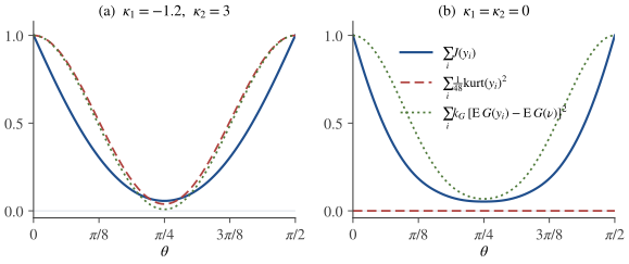
None of the approximations is accurate in absolute terms far from the Gaussian, which is not what they were designed for. The cumulant approximation overweights heavy tails (it gives $0.75$ for the $t_5$ law, sixteen times the true value) and returns zero for the zero-kurtosis mixture. The approximations with $G$ are of the right size for the three super-Gaussian laws (within about $20\%$ with $-e^{-u^2/2}$ , within a factor of $1.7$ with $\log\cosh$ ), react to the zero-kurtosis mixture, and underestimate strongly sub-Gaussian and skewed laws; an even $G$ cannot see skewness at all, so for skewed sources an odd function must be added. What matters for ICA, however, is how a contrast varies across the projections of one data set, and there the approximations follow the exact negentropy closely, as Figure 6.1图 6.1 shows.

在远离高斯的地方，这些近似的绝对数值都不准确，这本来也不是它们的设计目标。累积量近似过分看重重尾（对 $t_5$ 分布给出 $0.75$ ，是真值的十六倍），对峭度为零的混合则给出零。基于 $G$ 的近似对三个超高斯分布给出了量级正确的值（用 $-e^{-u^2/2}$ 时误差约在 $20\%$ 以内，用 $\log\cosh$ 时在 $1.7$ 倍以内），能对峭度为零的混合作出反应，但低估了强亚高斯分布与偏斜分布；偶函数 $G$ 完全看不见偏度，所以对偏斜的源必须再加一个奇函数项。不过，对 ICA 真正重要的是对比函数在同一组数据的不同投影之间如何变化，而在这一点上，这些近似紧紧跟随精确负熵，如Figure 6.1图 6.1所示。

Two panels plotting, against the rotation angle theta from 0 to pi/2, the sum of the marginal negentropies of two rotated sources together with two approximations, each divided by its value at theta = 0. Left: all three curves peak at theta = 0 and pi/2 and dip at pi/4. Right: the kurtosis-based curve is flat at zero, while the exact negentropy and the log cosh approximation still peak at 0 and pi/2. — **Figure 6.1.** Sum of the marginal negentropies of $\by = \bQ_\theta\bs$ , with $\bQ_\theta$ the rotation by $\theta$ , for two independent unit-variance sources; $\theta = 0$ and $\theta = \pi/2$ are the separating rotations. Solid: exact value, computed by numerical integration, which by Proposition 6.4命题 6.4 equals $J(\bz) - I(\by)$ . Dashed: the cumulant approximation (6.9). Dotted: the approximation (6.10) with $G = \log\cosh$ . Each curve is divided by its value at $\theta = 0$ , where the exact sums are $0.249$ and $0.147$ nats. (a) A uniform and a Laplacian source. (b) Two copies of the zero-kurtosis source: the kurtosis-based contrast is identically zero, whereas the exact negentropy and its $\log\cosh$ approximation are still maximized at separation.图 6.1 两个独立单位方差源经旋转 $\bQ_\theta$ （旋转角 $\theta$ ）后， $\by = \bQ_\theta\bs$ 各边缘负熵之和； $\theta = 0$ 与 $\theta = \pi/2$ 是分离旋转。实线：由数值积分得到的精确值，由Proposition 6.4命题 6.4它等于 $J(\bz) - I(\by)$ 。虚线：累积量近似 (6.9)。点线：取 $G = \log\cosh$ 的近似 (6.10)。每条曲线都除以其在 $\theta = 0$ 处的值，该处精确值分别为 $0.249$ 与 $0.147$ 奈特。（a）一个均匀源与一个拉普拉斯源。（b）峭度为零的源的两个独立副本：基于峭度的对比函数恒为零，而精确负熵及其 $\log\cosh$ 近似仍在分离处取最大值。

Why these approximations are more robust为什么这些近似更稳健

The advantages over kurtosis come from the slow growth of $G$ . First, variance: the sample average $\hat\E[G(y)]$ has variance $\Var(G(y))/T$ , which is finite as soon as $\E[G(y)^2] < \infty$ . Since $0 \le \log\cosh u \le |u|$ , a finite variance of $y$ suffices for $G = \log\cosh$ , and $-e^{-u^2/2}$ is bounded, so it needs no moment at all; the sample kurtosis needs $m_8 < \infty$ (Proposition 5.6命题 5.6). Second, influence: one observation $x_0$ moves $\hat\E[G(y)]$ by roughly $G(x_0)/T$ , which is at most about $|x_0|/T$ for $\log\cosh$ and at most $1/T$ for $-e^{-u^2/2}$ , against $x_0^4/T$ for the fourth moment. Third, sensitivity: they respond to departures from Gaussianity that leave the fourth moment unchanged. The following script compares the sample kurtosis with the $\log\cosh$ statistic on Gaussian data and on the zero-kurtosis source.

相对于峭度的优势来自 $G$ 的缓慢增长。其一是方差：样本平均 $\hat\E[G(y)]$ 的方差为 $\Var(G(y))/T$ ，只要 $\E[G(y)^2] < \infty$ 就有限。由于 $0 \le \log\cosh u \le |u|$ ，对 $G = \log\cosh$ 只需 $y$ 的方差有限； $-e^{-u^2/2}$ 有界，完全不需要矩条件；而样本峭度需要 $m_8 < \infty$ （Proposition 5.6命题 5.6）。其二是影响：单个观测 $x_0$ 使 $\hat\E[G(y)]$ 变化约 $G(x_0)/T$ ，对 $\log\cosh$ 至多约为 $|x_0|/T$ ，对 $-e^{-u^2/2}$ 至多为 $1/T$ ，而对四阶矩则是 $x_0^4/T$ 。其三是敏感性：它们能察觉不改变四阶矩的那些对高斯的偏离。下面的脚本在高斯数据和峭度为零的源上，比较样本峭度与 $\log\cosh$ 统计量。

import numpy as np

rng = np.random.default_rng(0)
T, runs = 10000, 300
EG_nu = 0.374567                          # E log cosh(nu), nu ~ N(0, 1)

def logcosh(u):
    return np.abs(u) + np.log1p(np.exp(-2 * np.abs(u))) - np.log(2)

def zero_kurtosis_source(size):
    """Uniform with probability 5/7, Laplacian with probability 2/7."""
    pick = rng.random(size) < 5 / 7
    return np.where(pick, rng.uniform(-np.sqrt(3), np.sqrt(3), size),
                    rng.laplace(0.0, 1 / np.sqrt(2), size))

sources = [("Gaussian", rng.standard_normal),
           ("zero-kurtosis", zero_kurtosis_source)]
for name, draw in sources:
    k, g = [], []
    for _ in range(runs):
        y = draw(T)
        y = (y - y.mean()) / y.std()              # standardize
        k.append(np.mean(y**4) - 3)               # sample kurtosis
        g.append(np.mean(logcosh(y)) - EG_nu)     # E G(y) - E G(nu)
    print(f"{name:14s} kurtosis {np.mean(k):+.3f} +/- {np.std(k):.3f}   "
          f"G-statistic {np.mean(g):+.4f} +/- {np.std(g):.4f}")

Over 300 samples of size $T = 10000$ , the sample kurtosis is $+0.003 \pm 0.049$ for Gaussian data and $+0.017 \pm 0.230$ for the zero-kurtosis source: kurtosis cannot tell them apart, and its spread is almost five times larger for the non-Gaussian law. The $\log\cosh$ statistic $\E G(y) - \E G(\nu)$ is $-0.0001 \pm 0.0008$ for the Gaussian and $+0.0087 \pm 0.0015$ for the zero-kurtosis source, a separation of about six standard deviations. (The logarithm is written in a form that does not overflow for large $|u|$ .)

对 300 个样本量为 $T = 10000$ 的样本，高斯数据的样本峭度为 $+0.003 \pm 0.049$ ，峭度为零的源为 $+0.017 \pm 0.230$ ：峭度区分不了二者，而且对这个非高斯分布，它的离散程度大了将近五倍。 $\log\cosh$ 统计量 $\E G(y) - \E G(\nu)$ 对高斯数据为 $-0.0001 \pm 0.0008$ ，对峭度为零的源为 $+0.0087 \pm 0.0015$ ，两者相差约六个标准差。（代码中对数的写法保证 $|u|$ 很大时也不会溢出。）

6.8 A map of contrast functions对比函数一览

Table 6.4表 6.4 collects the contrasts of Part II and the chapters where they are turned into algorithms. They fall into two families: those built on densities (mutual information, likelihood, Infomax, negentropy), which are linked by exact identities, and their moment-based or function-based approximations (kurtosis, cumulants, $G$ -functions). Hyvärinen, Karhunen & Oja (2001) give a textbook account of these contrasts and of the algorithms built on them.

Table 6.4表 6.4汇总了第二部分的对比函数，以及把它们变成算法的章节。它们分为两大类：基于密度的（互信息、似然、Infomax、负熵），彼此由精确恒等式联系；以及它们基于矩或基于函数 $G$ 的近似（峭度、累积量、 $G$ 函数）。Hyvärinen, Karhunen & Oja（2001）对这些对比函数以及由此构造的算法有系统的教科书式论述。

Table 6.4. Contrast functions for ICA. "Rotations" means that the criterion is optimized over orthogonal

\bU

after whitening.表 6.4 ICA 的对比函数。“旋转”指在白化之后对正交矩阵

\bU

优化该准则。

Contrast对比函数	Criterion准则	Properties性质	Chapters章
Mutual information互信息	$\min\ I(\by) = \sum_i H(y_i) - H(\by)$	exact measure of dependence; minima are the separating matrices (at most one Gaussian); needs marginal densities相依性的精确度量；最小点即分离矩阵（至多一个高斯源）；需要边缘密度	$4, 6$
Likelihood似然	$\max\ \sum_i \E\log p_i(y_i) + \log\|\det\bW\|$	equals $-H(\bx) - I(\by) - \sum_i D(p_{y_i}\\|p_i)$ ; separation is always stationary; stability needs a model of the right sub- or super-Gaussian type等于 $-H(\bx) - I(\by) - \sum_i D(p_{y_i}\\|p_i)$ ；分离解总是驻点；稳定性要求模型属于正确的亚高斯或超高斯类型	$6, 7, 10$
InfomaxInfomax	$\max\ H\bigl(\mathbf{g}(\bW\bx)\bigr)$	maximum likelihood with model densities $g_i'$ ; logistic $g$ is a super-Gaussian model以 $g_i'$ 为模型密度的最大似然；logistic 函数对应超高斯模型	$6, 7$
Sum of negentropies负熵之和	$\max\ \sum_i J(y_i)$ , rotations，旋转	equals $J(\bz) - I(\by)$ ; needs marginal densities等于 $J(\bz) - I(\by)$ ；需要边缘密度	$6$
Negentropy approximation负熵近似	$\max\ [\E G(\bw^\top\bz) - \E G(\nu)]^2$	one unit at a time; robust for slowly growing $G$ such as $\log\cosh$ or $-e^{-u^2/2}$ 一次提取一个单元； $G$ 增长缓慢（如 $\log\cosh$ 或 $-e^{-u^2/2}$ ）时稳健	$6, 8$
Absolute kurtosis峭度绝对值	$\max\ \|\kurt(\bw^\top\bz)\|$	no spurious local maxima; sensitive to outliers and heavy tails; blind to zero-kurtosis sources没有伪局部极大点；对离群值与重尾敏感；看不见峭度为零的源	$5, 8$
Sum of squared kurtoses峭度平方和	$\max\ \sum_i \kurt(y_i)^2$ , rotations，旋转	global maxima are the separating rotations if at most one source has zero kurtosis; equivalent to minimizing squared fourth-order cross-cumulants若至多一个源的峭度为零，全局最大点就是分离旋转；等价于最小化四阶交叉累积量的平方和	$5, 9$

Key points

本章要点

The change of variables gives the likelihood $\log L(\bW) = \sum_t\sum_i \log p_i(\bw_i^\top\bx(t)) + T\log|\det\bW|$ ; its stationary points solve the estimating equations $\E[\varphi_i(y_i)y_j] = \delta_{ij}$ , with $\varphi_i = -p_i'/p_i$ the model scores.
Exactly, $\mathcal{L}(\bW) = -H(\bx) - I(\by) - \sum_i D(p_{y_i}\|p_i)$ : maximum likelihood minimizes the dependence of the outputs plus the mismatch of their marginals with the model.
For whitened data and rotations, $I(\by) = J(\bz) - \sum_i J(y_i)$ : minimizing dependence is maximizing the non-Gaussianity of the outputs.
Infomax with squashing functions $g_i$ is maximum likelihood with model densities $g_i'$ ; the logistic choice is a super-Gaussian model.
Separation solves the estimating equations for any source model, after rescaling; only its stability depends on the model, through the conditions $\gamma_i > 0$ and $\gamma_i\gamma_j > 1$ for every pair. The true score is always stable when at most one source is Gaussian, while a fixed sub- or super-Gaussian model can fail, which is why models are switched per output.
Negentropy can be approximated by $\frac1{12}\kappa_3^2 + \frac1{48}\kappa_4^2$ , which inherits the weaknesses of kurtosis, or by $k_G[\E G(y) - \E G(\nu)]^2$ with $\log\cosh$ or $-e^{-u^2/2}$ , which needs weaker moment conditions, limits the influence of outliers and sees beyond the fourth moment.

变量替换给出似然 $\log L(\bW) = \sum_t\sum_i \log p_i(\bw_i^\top\bx(t)) + T\log|\det\bW|$ ；其驻点满足估计方程 $\E[\varphi_i(y_i)y_j] = \delta_{ij}$ ，其中 $\varphi_i = -p_i'/p_i$ 是模型得分函数。
精确地有 $\mathcal{L}(\bW) = -H(\bx) - I(\by) - \sum_i D(p_{y_i}\|p_i)$ ：最大似然最小化的是输出的相依性加上其边缘分布与模型的失配。
对白化数据与旋转， $I(\by) = J(\bz) - \sum_i J(y_i)$ ：最小化相依性就是最大化输出的非高斯性。
以 $g_i$ 为压缩函数的 Infomax 就是以 $g_i'$ 为模型密度的最大似然；logistic 函数对应超高斯模型。
经过尺度调整后，分离解对任何源模型都满足估计方程；只有它的稳定性依赖于模型，由条件 $\gamma_i > 0$ 以及对每一对源的 $\gamma_i\gamma_j > 1$ 决定。至多一个源是高斯时，真实得分函数总是稳定的；固定的亚高斯或超高斯模型则可能失败，这就是要为每个输出切换模型的原因。
负熵可以用 $\frac1{12}\kappa_3^2 + \frac1{48}\kappa_4^2$ 近似，它继承了峭度的弱点；也可以用 $k_G[\E G(y) - \E G(\nu)]^2$ （取 $\log\cosh$ 或 $-e^{-u^2/2}$ ）近似，后者只需较弱的矩条件，限制了离群值的影响，并能看到四阶矩以外的信息。

6.9 Exercises习题

Exercise 6.1习题 6.1 basic基础

(a) Compute the score of the unit-variance Laplace density $p(u) = \frac{1}{\sqrt2}e^{-\sqrt2|u|}$ , and verify $\E[\psi(s)s] = 1$ and $\mathcal{J} = 2$ . (b) Show that the score of the logistic density $e^{-u}/(1+e^{-u})^2$ is $\tanh(u/2)$ and that the score of $1/(\pi\cosh u)$ is $\tanh u$ .

（a）求单位方差拉普拉斯密度 $p(u) = \frac{1}{\sqrt2}e^{-\sqrt2|u|}$ 的得分函数，并验证 $\E[\psi(s)s] = 1$ 与 $\mathcal{J} = 2$ 。（b）证明 logistic 密度 $e^{-u}/(1+e^{-u})^2$ 的得分函数为 $\tanh(u/2)$ ，而 $1/(\pi\cosh u)$ 的得分函数为 $\tanh u$ 。

Show solution查看解答

(a) $\log p(u) = -\frac12\log 2 - \sqrt2|u|$ , so $\psi(u) = \sqrt2\,\sign(u)$ for $u \neq 0$ . The mean absolute value of a Laplace variable equals its scale, here $1/\sqrt2$ , so $\E[\psi(s)s] = \sqrt2\,\E|s| = 1$ , and $\mathcal{J} = \E[\psi(s)^2] = 2$ , which exceeds the Gaussian value $1$ . (b) For the logistic density, $\log p(u) = -u - 2\log(1 + e^{-u})$ , whose derivative is $-1 + 2e^{-u}/(1 + e^{-u}) = -(1 - e^{-u})/(1 + e^{-u}) = -\tanh(u/2)$ ; hence $\psi(u) = \tanh(u/2)$ . For the hyperbolic secant density, $\log p(u) = -\log\pi - \log\cosh u$ , whose derivative is $-\tanh u$ , so $\psi(u) = \tanh u$ . Both scores saturate, as befits super-Gaussian densities.

（a） $\log p(u) = -\frac12\log 2 - \sqrt2|u|$ ，所以 $u \neq 0$ 时 $\psi(u) = \sqrt2\,\sign(u)$ 。拉普拉斯变量的平均绝对值等于其尺度参数，这里为 $1/\sqrt2$ ，故 $\E[\psi(s)s] = \sqrt2\,\E|s| = 1$ ，且 $\mathcal{J} = \E[\psi(s)^2] = 2$ ，大于高斯分布的取值 $1$ 。（b）对 logistic 密度， $\log p(u) = -u - 2\log(1 + e^{-u})$ ，其导数为 $-1 + 2e^{-u}/(1 + e^{-u}) = -(1 - e^{-u})/(1 + e^{-u}) = -\tanh(u/2)$ ，因此 $\psi(u) = \tanh(u/2)$ 。对双曲正割密度， $\log p(u) = -\log\pi - \log\cosh u$ ，其导数为 $-\tanh u$ ，所以 $\psi(u) = \tanh u$ 。两个得分函数都是饱和的，这与超高斯密度相符。

Exercise 6.2习题 6.2 basic基础

Show that $I(\bD\by) = I(\by)$ for every invertible diagonal $\bD$ , whereas $\mathcal{L}(\bD\bW)$ depends on $\bD$ . Show that the condition $\partial\mathcal{L}(\bD\bW)/\partial d_i = 0$ at $\bD = \bI$ is the diagonal estimating equation $\E[\varphi_i(y_i)y_i] = 1$ .

证明对任意可逆对角矩阵 $\bD$ 都有 $I(\bD\by) = I(\by)$ ，而 $\mathcal{L}(\bD\bW)$ 依赖于 $\bD$ 。证明在 $\bD = \bI$ 处 $\partial\mathcal{L}(\bD\bW)/\partial d_i = 0$ 恰好就是对角估计方程 $\E[\varphi_i(y_i)y_i] = 1$ 。

Show solution查看解答

$H(d_i y_i) = H(y_i) + \log|d_i|$ and $H(\bD\by) = H(\by) + \sum_i\log|d_i|$ , so the logarithms cancel in $I(\bD\by) = \sum_i H(d_iy_i) - H(\bD\by)$ . On the other hand $\mathcal{L}(\bD\bW) = \sum_i \E[\log p_i(d_i y_i)] + \log|\det\bW| + \sum_i \log|d_i|$ , which changes with $\bD$ unless the $p_i$ have a special form. Its derivative with respect to $d_i$ is $-\E[\varphi_i(d_iy_i)\,y_i] + 1/d_i$ , which at $d_i = 1$ vanishes exactly when $\E[\varphi_i(y_i)y_i] = 1$ . The diagonal estimating equations therefore only fix the scales of the outputs, the one thing that mutual information ignores; the off-diagonal equations carry the information about independence.

$H(d_i y_i) = H(y_i) + \log|d_i|$ ， $H(\bD\by) = H(\by) + \sum_i\log|d_i|$ ，所以在 $I(\bD\by) = \sum_i H(d_iy_i) - H(\bD\by)$ 中这些对数项相互抵消。另一方面， $\mathcal{L}(\bD\bW) = \sum_i \E[\log p_i(d_i y_i)] + \log|\det\bW| + \sum_i \log|d_i|$ ，除非 $p_i$ 具有特殊形式，否则它随 $\bD$ 变化。它对 $d_i$ 的导数为 $-\E[\varphi_i(d_iy_i)\,y_i] + 1/d_i$ ，在 $d_i = 1$ 处为零当且仅当 $\E[\varphi_i(y_i)y_i] = 1$ 。因此对角估计方程只确定输出的尺度，而这恰恰是互信息所不关心的；关于独立性的信息由非对角方程承载。

Exercise 6.3习题 6.3 intermediate进阶

Let $\gamma = \E[\varphi'(y)]\,\E[y^2]$ , evaluated at the scale $y = ds$ that solves the scale equation (6.8). (a) For $\varphi(u) = u^3$ and a unit-variance source with kurtosis $\kappa$ , show that $\gamma = 3/(3 + \kappa)$ . (b) Show that $\gamma = 1$ for a Gaussian source and every differentiable $\varphi$ with $\E|\varphi'(y)| < \infty$ , using Stein's identity $\E[\varphi(y)\,y] = \sigma^2\E[\varphi'(y)]$ for $y \sim \Ncal(0, \sigma^2)$ , and prove that identity. (c) Show that with the true score, $\gamma = \mathcal{J}\sigma^2 \ge 1$ .

令 $\gamma = \E[\varphi'(y)]\,\E[y^2]$ ，在使尺度方程 (6.8) 成立的尺度 $y = ds$ 处计算。（a）对 $\varphi(u) = u^3$ 与峭度为 $\kappa$ 的单位方差源，证明 $\gamma = 3/(3 + \kappa)$ 。（b）利用 $y \sim \Ncal(0, \sigma^2)$ 时的 Stein 恒等式 $\E[\varphi(y)\,y] = \sigma^2\E[\varphi'(y)]$ ，证明对高斯源以及任意满足 $\E|\varphi'(y)| < \infty$ 的可微函数 $\varphi$ 都有 $\gamma = 1$ ，并证明该恒等式。（c）证明用真实得分函数时 $\gamma = \mathcal{J}\sigma^2 \ge 1$ 。

Show solution查看解答

(a) The scale equation reads $\E[(ds)^3\, ds] = d^4\E[s^4] = d^4(3 + \kappa) = 1$ . Then $\gamma = \E[3(ds)^2]\cdot\E[(ds)^2] = 3d^2 \cdot d^2 = 3d^4 = 3/(3 + \kappa)$ : above $1$ for sub-Gaussian and below $1$ for super-Gaussian sources. (b) The Gaussian density $\phi_\sigma$ satisfies $u\,\phi_\sigma(u) = -\sigma^2\phi_\sigma'(u)$ , so integrating by parts, $\E[\varphi(y)y] = -\sigma^2\int\varphi\,\phi_\sigma' = \sigma^2\int\varphi'\,\phi_\sigma = \sigma^2\E[\varphi'(y)]$ , the boundary terms vanishing because $\phi_\sigma$ decays faster than any polynomial (we also assume $\varphi\,\phi_\sigma \to 0$ at infinity). At the separating scale $\E[\varphi(y)y] = 1$ , hence $\gamma = \E[\varphi'(y)]\,\sigma^2 = \E[\varphi(y)y] = 1$ . (c) With the true score $\psi$ of $s$ , the scale equation holds at $d = 1$ because $\E[\psi(s)s] = 1$ (Section 6.2第 6.2 节), and $\E[\psi'(s)] = \E[\psi(s)^2] = \mathcal{J}$ . Thus $\gamma = \mathcal{J}\sigma^2$ , and the Cauchy–Schwarz inequality $1 = \E[\psi(s)s]^2 \le \mathcal{J}\sigma^2$ gives $\gamma \ge 1$ , with equality only for a Gaussian source.

（a）尺度方程为 $\E[(ds)^3\, ds] = d^4\E[s^4] = d^4(3 + \kappa) = 1$ 。于是 $\gamma = \E[3(ds)^2]\cdot\E[(ds)^2] = 3d^2 \cdot d^2 = 3d^4 = 3/(3 + \kappa)$ ：对亚高斯源大于 $1$ ，对超高斯源小于 $1$ 。（b）高斯密度 $\phi_\sigma$ 满足 $u\,\phi_\sigma(u) = -\sigma^2\phi_\sigma'(u)$ ，分部积分得 $\E[\varphi(y)y] = -\sigma^2\int\varphi\,\phi_\sigma' = \sigma^2\int\varphi'\,\phi_\sigma = \sigma^2\E[\varphi'(y)]$ ；由于 $\phi_\sigma$ 衰减得比任何多项式都快，边界项为零（这里还假定在无穷远处 $\varphi\,\phi_\sigma \to 0$ ）。在分离尺度处 $\E[\varphi(y)y] = 1$ ，因此 $\gamma = \E[\varphi'(y)]\,\sigma^2 = \E[\varphi(y)y] = 1$ 。（c）用 $s$ 的真实得分函数 $\psi$ 时，由于 $\E[\psi(s)s] = 1$ （Section 6.2第 6.2 节），尺度方程在 $d = 1$ 处成立，且 $\E[\psi'(s)] = \E[\psi(s)^2] = \mathcal{J}$ 。于是 $\gamma = \mathcal{J}\sigma^2$ ，而 Cauchy–Schwarz 不等式 $1 = \E[\psi(s)s]^2 \le \mathcal{J}\sigma^2$ 给出 $\gamma \ge 1$ ，等号只对高斯源成立。

Exercise 6.4习题 6.4 intermediate进阶

For $G(u) = -e^{-u^2/2}$ , compute $\E G(\nu)$ , $\Var G(\nu)$ and $\Cov(G(\nu), \nu^2)$ , and show that $k_G = 24/(16\sqrt3 - 27) \approx 33.67$ . (Hint: $\E[e^{-a\nu^2}] = (1 + 2a)^{-1/2}$ and $\E[\nu^2 e^{-a\nu^2}] = (1 + 2a)^{-3/2}$ for $a > -1/2$ .)

对 $G(u) = -e^{-u^2/2}$ ，计算 $\E G(\nu)$ 、 $\Var G(\nu)$ 与 $\Cov(G(\nu), \nu^2)$ ，并证明 $k_G = 24/(16\sqrt3 - 27) \approx 33.67$ 。（提示：当 $a > -1/2$ 时， $\E[e^{-a\nu^2}] = (1 + 2a)^{-1/2}$ ， $\E[\nu^2 e^{-a\nu^2}] = (1 + 2a)^{-3/2}$ 。）

Show solution查看解答

With $a = 1/2$ : $\E G(\nu) = -2^{-1/2}$ and $\E[\nu^2 G(\nu)] = -2^{-3/2}$ ; with $a = 1$ : $\E[G(\nu)^2] = \E[e^{-\nu^2}] = 3^{-1/2}$ . Hence $\Var G(\nu) = 1/\sqrt3 - 1/2$ and $\Cov(G(\nu), \nu^2) = -2^{-3/2} + 2^{-1/2} = 2^{-3/2}$ , whose square is $1/8$ . Therefore $c_G^2 = 1/\sqrt3 - 1/2 - 1/16 = 1/\sqrt3 - 9/16 \approx 0.01485$ and $k_G = 1/(2c_G^2) = 1/(2/\sqrt3 - 9/8) = 8\sqrt3/(16 - 9\sqrt3) = 24/(16\sqrt3 - 27) \approx 33.67$ , where the last step multiplies numerator and denominator by $\sqrt3$ . The small value of $c_G^2$ means that $G(\nu)$ is almost a quadratic function of $\nu$ in the $L^2(\phi)$ sense, so small deviations of $\E G(y)$ from $\E G(\nu)$ already signal substantial negentropy.

取 $a = 1/2$ ： $\E G(\nu) = -2^{-1/2}$ ， $\E[\nu^2 G(\nu)] = -2^{-3/2}$ ；取 $a = 1$ ： $\E[G(\nu)^2] = \E[e^{-\nu^2}] = 3^{-1/2}$ 。因此 $\Var G(\nu) = 1/\sqrt3 - 1/2$ ， $\Cov(G(\nu), \nu^2) = -2^{-3/2} + 2^{-1/2} = 2^{-3/2}$ ，其平方为 $1/8$ 。于是 $c_G^2 = 1/\sqrt3 - 1/2 - 1/16 = 1/\sqrt3 - 9/16 \approx 0.01485$ ， $k_G = 1/(2c_G^2) = 1/(2/\sqrt3 - 9/8) = 8\sqrt3/(16 - 9\sqrt3) = 24/(16\sqrt3 - 27) \approx 33.67$ ，最后一步是把分子分母同乘 $\sqrt3$ 。 $c_G^2$ 很小，说明在 $L^2(\phi)$ 意义下 $G(\nu)$ 几乎是 $\nu$ 的二次函数，因此 $\E G(y)$ 与 $\E G(\nu)$ 之间的微小偏差就已意味着可观的负熵。

Exercise 6.5习题 6.5 advanced硬核

Let $y$ have zero mean, unit variance, and third and fourth cumulants $\kappa_3, \kappa_4$ , and suppose its density is $p = \phi(1 + \varepsilon)$ with $\varepsilon = \frac{\kappa_3}{6}H_3 + \frac{\kappa_4}{24}H_4$ , a small correction. (a) Check that $p$ has the stated moments up to order four, using $\int \phi\, H_j H_k = k!\,\delta_{jk}$ . (b) Derive (6.9) from $J(y) = D(p\|\phi)$ by expanding $\log(1 + \varepsilon)$ to second order.

设 $y$ 均值为零、方差为一，三阶与四阶累积量为 $\kappa_3, \kappa_4$ ，并设其密度为 $p = \phi(1 + \varepsilon)$ ，其中 $\varepsilon = \frac{\kappa_3}{6}H_3 + \frac{\kappa_4}{24}H_4$ 是小的修正项。（a）利用 $\int \phi\, H_j H_k = k!\,\delta_{jk}$ ，验证 $p$ 直到四阶的矩与所述相符。（b）由 $J(y) = D(p\|\phi)$ 出发，把 $\log(1 + \varepsilon)$ 展开到二阶，推导 (6.9)。

Show solution查看解答

(a) The monomials $1, u, u^2$ are combinations of $H_0, H_1, H_2$ , which are orthogonal to $H_3$ and $H_4$ , so $p$ integrates to one and has the mean $0$ and variance $1$ of $\phi$ . Since $u^3 = H_3 + 3H_1$ , $\int u^3 p = \frac{\kappa_3}{6}\int\phi H_3^2 = \frac{\kappa_3}{6}\cdot 3! = \kappa_3$ ; the $H_4$ term contributes nothing by parity. Since $u^4 = H_4 + 6H_2 + 3H_0$ , $\int u^4 p = 3 + \frac{\kappa_4}{24}\cdot 4! = 3 + \kappa_4$ , so the fourth cumulant is $\kappa_4$ . (b) $D(p\|\phi) = \int \phi(1+\varepsilon)\log(1+\varepsilon)$ . With $\log(1+\varepsilon) = \varepsilon - \frac12\varepsilon^2 + O(\varepsilon^3)$ , we get $(1+\varepsilon)\log(1+\varepsilon) = \varepsilon + \frac12\varepsilon^2 + O(\varepsilon^3)$ . The first term integrates to zero against $\phi$ by orthogonality to $H_0$ , and by orthogonality of $H_3$ and $H_4$ ,

（a）单项式 $1, u, u^2$ 都是 $H_0, H_1, H_2$ 的线性组合，与 $H_3$ 、 $H_4$ 正交，所以 $p$ 的积分为一，且具有 $\phi$ 的均值 $0$ 与方差 $1$ 。由 $u^3 = H_3 + 3H_1$ ， $\int u^3 p = \frac{\kappa_3}{6}\int\phi H_3^2 = \frac{\kappa_3}{6}\cdot 3! = \kappa_3$ ；由奇偶性， $H_4$ 项没有贡献。由 $u^4 = H_4 + 6H_2 + 3H_0$ ， $\int u^4 p = 3 + \frac{\kappa_4}{24}\cdot 4! = 3 + \kappa_4$ ，所以四阶累积量为 $\kappa_4$ 。（b） $D(p\|\phi) = \int \phi(1+\varepsilon)\log(1+\varepsilon)$ 。由 $\log(1+\varepsilon) = \varepsilon - \frac12\varepsilon^2 + O(\varepsilon^3)$ 得 $(1+\varepsilon)\log(1+\varepsilon) = \varepsilon + \frac12\varepsilon^2 + O(\varepsilon^3)$ 。第一项与 $\phi$ 相乘后积分为零（与 $H_0$ 正交）；由 $H_3$ 与 $H_4$ 的正交性，

J(y) \approx \frac12\int\phi\,\varepsilon^2 = \frac12\Bigl(\frac{\kappa_3^2}{36}\cdot 3! + \frac{\kappa_4^2}{576}\cdot 4!\Bigr) = \frac{\kappa_3^2}{12} + \frac{\kappa_4^2}{48}.

This is the same result as (6.10) with $G = u^3$ and $G = u^4$ : the normalized Hermite polynomials $H_3/\sqrt{6}$ and $H_4/\sqrt{24}$ are exactly the orthonormalized versions of $u^3$ and $u^4$ , and their expectations under $y$ are $\kappa_3/\sqrt6$ and $\kappa_4/\sqrt{24}$ .

这与在 (6.10) 中取 $G = u^3$ 与 $G = u^4$ 的结果相同：归一化的 Hermite 多项式 $H_3/\sqrt{6}$ 与 $H_4/\sqrt{24}$ 恰好是 $u^3$ 与 $u^4$ 经正交归一化后的形式，它们在 $y$ 下的期望分别为 $\kappa_3/\sqrt6$ 与 $\kappa_4/\sqrt{24}$ 。

Exercise 6.6习题 6.6 advanced硬核

The entropy power inequality states that for independent random variables $X$ and $Y$ with densities and finite variances, $e^{2H(X+Y)} \ge e^{2H(X)} + e^{2H(Y)}$ , with equality only if $X$ and $Y$ are Gaussian (Cover & Thomas, 2006). Let $\bs$ have independent unit-variance components with densities, and let $y = \bq^\top\bs$ with $\|\bq\| = 1$ . Show that $J(y) \le \max_i J(s_i)$ , and that if some source is non-Gaussian, equality holds only for $\bq = \pm\be_i$ with $J(s_i) = \max_j J(s_j)$ .

熵幂不等式断言：对具有密度且方差有限的独立随机变量 $X$ 与 $Y$ ， $e^{2H(X+Y)} \ge e^{2H(X)} + e^{2H(Y)}$ ，等号仅当 $X$ 与 $Y$ 都是高斯时成立（Cover & Thomas, 2006）。设 $\bs$ 的各分量独立、方差为一且有密度，令 $y = \bq^\top\bs$ ， $\|\bq\| = 1$ 。证明 $J(y) \le \max_i J(s_i)$ ；并证明若有某个源非高斯，则等号仅在 $\bq = \pm\be_i$ 且 $J(s_i) = \max_j J(s_j)$ 时成立。

Show solution查看解答

By induction the inequality extends to finite sums of independent variables, $e^{2H(\sum_i X_i)} \ge \sum_i e^{2H(X_i)}$ , with equality only if all $X_i$ are Gaussian. Apply it to $X_i = q_i s_i$ for the indices with $q_i \neq 0$ . Since $H(q_i s_i) = H(s_i) + \log|q_i|$ , we have $e^{2H(X_i)} = q_i^2 e^{2H(s_i)}$ . All the variables involved have unit variance, so $H(\cdot) = h - J(\cdot)$ with $h = \frac12\log(2\pi e)$ , and the inequality becomes $e^{-2J(y)} \ge \sum_i q_i^2 e^{-2J(s_i)}$ . Since the weights $q_i^2$ sum to one, the right side is at least $e^{-2\max_i J(s_i)}$ , hence $J(y) \le \max_i J(s_i)$ . If two or more $q_i$ are nonzero, equality would require equality in the entropy power inequality, hence Gaussian $s_i$ for those indices, and then $J(y) = 0$ ; so if $\max_j J(s_j) > 0$ , equality forces $\bq = \pm\be_i$ , and then $J(y) = J(s_i)$ must be the maximum. In whitened coordinates, the global maximum of $J(\bw^\top\bz)$ on the sphere is therefore attained exactly at the sources of largest negentropy. The argument says nothing about other local maxima; unlike Theorem 5.3定理 5.3, it does not rule them out.

由归纳法，该不等式可推广到有限个独立变量之和： $e^{2H(\sum_i X_i)} \ge \sum_i e^{2H(X_i)}$ ，等号仅当所有 $X_i$ 都是高斯时成立。对满足 $q_i \neq 0$ 的下标取 $X_i = q_i s_i$ 。由 $H(q_i s_i) = H(s_i) + \log|q_i|$ 得 $e^{2H(X_i)} = q_i^2 e^{2H(s_i)}$ 。所涉及的变量方差都为一，所以 $H(\cdot) = h - J(\cdot)$ ，其中 $h = \frac12\log(2\pi e)$ ，不等式变为 $e^{-2J(y)} \ge \sum_i q_i^2 e^{-2J(s_i)}$ 。由于权重 $q_i^2$ 之和为一，右边至少为 $e^{-2\max_i J(s_i)}$ ，因此 $J(y) \le \max_i J(s_i)$ 。若有两个或更多 $q_i$ 非零，取等号就要求熵幂不等式取等号，从而这些下标对应的 $s_i$ 都是高斯的，此时 $J(y) = 0$ ；所以当 $\max_j J(s_j) > 0$ 时，等号迫使 $\bq = \pm\be_i$ ，而此时 $J(y) = J(s_i)$ 必须是最大值。换到白化坐标下， $J(\bw^\top\bz)$ 在球面上的全局最大值恰好在负熵最大的源处取得。这一论证对其他局部极大点只字未提；与Theorem 5.3定理 5.3不同，它并不排除它们的存在。

6.10 References参考文献

Bell, A. J., & Sejnowski, T. J. (1995). An information-maximization approach to blind separation and blind deconvolution. Neural Computation, 7(6), 1129–1159.
Cardoso, J.-F. (1997). Infomax and maximum likelihood for blind source separation. IEEE Signal Processing Letters, 4(4), 112–114.
Cardoso, J.-F. (1998). Blind signal separation: Statistical principles. Proceedings of the IEEE, 86(10), 2009–2025.
Comon, P. (1994). Independent component analysis, a new concept? Signal Processing, 36(3), 287–314.
Cover, T. M., & Thomas, J. A. (2006). Elements of Information Theory (2nd ed.). Wiley.
Hyvärinen, A. (1998). New approximations of differential entropy for independent component analysis and projection pursuit. In Advances in Neural Information Processing Systems 10 (pp. 273–279). MIT Press.
Hyvärinen, A. (1999). Fast and robust fixed-point algorithms for independent component analysis. IEEE Transactions on Neural Networks, 10(3), 626–634.
Hyvärinen, A., Karhunen, J., & Oja, E. (2001). Independent Component Analysis. Wiley.
Jones, M. C., & Sibson, R. (1987). What is projection pursuit? Journal of the Royal Statistical Society, Series A, 150(1), 1–36.
Lee, T.-W., Girolami, M., & Sejnowski, T. J. (1999). Independent component analysis using an extended infomax algorithm for mixed subgaussian and supergaussian sources. Neural Computation, 11(2), 417–441.
Pearlmutter, B. A., & Parra, L. C. (1997). Maximum likelihood blind source separation: A context-sensitive generalization of ICA. In Advances in Neural Information Processing Systems 9 (pp. 613–619). MIT Press.
Pham, D.-T., & Garat, P. (1997). Blind separation of mixture of independent sources through a quasi-maximum likelihood approach. IEEE Transactions on Signal Processing, 45(7), 1712–1725.