Overcomplete ICA and Sparse Component Analysis过完备 ICA 与稀疏成分分析

12.1 More sources than sensors源多于传感器

Two microphones in a room with three speakers, a few dozen EEG electrodes picking up many more cortical sources, a pair of stereo channels carrying a whole band: in each case there are more sources than sensors. The model is still (1.1), $\bx = \bA\bs$, but now $\bA \in \R^{m \times n}$ with $m < n$. Such a mixture is called overcomplete, since $\bA$ has more columns than the dimension of the space they live in, or underdetermined, since $\bx = \bA\bs$ has fewer equations than unknowns. Throughout the chapter $\bA$ has rank $m$ and no zero column.

屋里有三个人说话却只有两只麦克风；几十个 EEG 电极接收到远多于此的皮层源；两个立体声声道承载着整支乐队：这些情形下源都多于传感器。模型仍是 (1.1)，即 $\bx = \bA\bs$，但此时 $\bA \in \R^{m \times n}$ 且 $m < n$。这样的混合称为过完备的，因为 $\bA$ 的列数多于它们所在空间的维数；也称为欠定的，因为方程 $\bx = \bA\bs$ 的方程个数少于未知数个数。本章始终假设 $\bA$ 的秩为 $m$，且没有零列。

In the square case two questions have the same answer: can $\bA$ be identified from the distribution of $\bx$, and can the sources be recovered from the observations? With $m < n$ they separate. The first answer is still yes, under conditions close to those of Comon's theorem (Section 12.2第 12.2 节). The second is no: even with $\bA$ known, $\bs(t)$ cannot be computed from $\bx(t)$, and it can be estimated well only with prior information such as sparsity (Section 12.3第 12.3 节). The chapter then turns to how $\bA$ can actually be estimated, from cumulant tensors (Section 12.4第 12.4 节) or from sparsity (Section 12.5第 12.5 节), and to why the problem is harder than square ICA (Section 12.6第 12.6 节).

在方阵情形下，两个问题的答案相同：能否从 $\bx$ 的分布辨识出 $\bA$？能否从观测中恢复出源？当 $m < n$ 时，这两个问题分道扬镳。第一个问题的答案仍然是肯定的，条件与 Comon 定理相近（Section 12.2第 12.2 节）。第二个问题的答案是否定的：即使 $\bA$ 已知，也无法由 $\bx(t)$ 算出 $\bs(t)$，只有借助稀疏性之类的先验信息才能把它估计好（Section 12.3第 12.3 节）。随后本章讨论 $\bA$ 实际上怎样估计：利用累积量张量（Section 12.4第 12.4 节）或利用稀疏性（Section 12.5第 12.5 节）；最后说明这个问题为什么比方阵 ICA 更难（Section 12.6第 12.6 节）。

12.2 What is still identifiable仍然可辨识的是什么

Two columns that are collinear, $\ba_2 = c\,\ba_1$, can never be told apart, because $s_1\ba_1 + s_2\ba_2 = (s_1 + cs_2)\,\ba_1$ behaves like a single source. Apart from this, non-Gaussianity pins down every column, however many there are.

两个共线的列 $\ba_2 = c\,\ba_1$ 永远无法区分，因为 $s_1\ba_1 + s_2\ba_2 = (s_1 + cs_2)\,\ba_1$ 的表现与单个源无异。除此之外，非高斯性能确定每一列，无论列有多少。

Part 1 is a theorem of Kagan, Linnik and Rao (1973) on the uniqueness of linear structures, which holds without any moment conditions; Eriksson and Koivunen (2004) used it to separate identifiability, separability and uniqueness in ICA. We prove it under the extra assumption that the sources have moment generating functions near zero, with the same tools as the Darmois–Skitovich theorem (Theorem 4.2定理 4.2). The key step is a lemma on powers of linear forms.

第 1 部分是 Kagan、Linnik 和 Rao（1973）关于线性结构唯一性的一个定理，它不需要任何矩条件；Eriksson 和 Koivunen（2004）用它厘清了 ICA 中可辨识性、可分离性与唯一性的区别。下面在源的矩母函数在零点附近存在这一额外假设下给出证明，所用工具与 Darmois–Skitovich 定理（Theorem 4.2定理 4.2）相同。关键一步是一个关于线性型之幂的引理。

Three remarks delimit the result. First, it says nothing about the columns of Gaussian sources, and part 2 genuinely needs the non-Gaussianity of both representations: if two sources contain independent Gaussian parts, those parts can be rotated into new directions, giving a second representation with two extra Gaussian columns (Exercise 12.5习题 12.5). Second, identifiability of $\bA$ does not identify the sources: under further conditions on the characteristic functions the distribution of $\bs$ is determined as well (Eriksson & Koivunen, 2004), but the values $\bs(t)$ never are (next section). Third, identifiability is a statement about the whole distribution of $\bx$; Section 12.4第 12.4 节 shows that low-order statistics may not suffice.

有三点说明界定了这个结果的范围。其一，它对高斯源的列不作任何断言，而且第 2 部分确实需要两个表示都是非高斯的：若有两个源各含一个独立的高斯部分，这两个高斯部分可以被旋转到新的方向上，从而得到多出两个高斯列的第二个表示（Exercise 12.5习题 12.5）。其二，$\bA$ 可辨识并不意味着源可辨识：在关于特征函数的进一步条件下，$\bs$ 的分布也被确定（Eriksson & Koivunen, 2004），但取值 $\bs(t)$ 永远无法确定（见下一节）。其三，可辨识性说的是 $\bx$ 的整个分布；Section 12.4第 12.4 节将说明低阶统计量可能不够用。

12.3 Recovering the sources恢复源

Suppose $\bA$ is known. In the square case $\bs = \bA^{-1}\bx$. With $m < n$ no such formula exists.

假设 $\bA$ 已知。在方阵情形下 $\bs = \bA^{-1}\bx$；当 $m < n$ 时，不存在这样的公式。

Every point of the solution set explains the observation equally well, so the choice among them must come from prior knowledge of the sources. With independent source densities $p_i$, the maximum a posteriori (MAP) estimate in the noiseless model, and its version for Gaussian noise of variance $\sigma^2$, are

解集中的每一点都同样好地解释了观测，所以只能依靠关于源的先验知识在其中作选择。若源的密度为相互独立的 $p_i$，无噪声模型中的最大后验（MAP）估计，以及方差为 $\sigma^2$ 的高斯噪声下的相应形式为

A Gaussian prior gives the minimum-norm solution $\bA^{+}\bx$, which spreads energy over all sources. A Laplace prior, $\log p_i(s) = -|s|/b + \text{const}$, turns the noiseless problem into

高斯先验给出最小范数解 $\bA^{+}\bx$，它把能量分摊到所有源上。拉普拉斯先验 $\log p_i(s) = -|s|/b + \text{常数}$ 则把无噪声问题变为

the basis pursuit problem of Chen, Donoho and Saunders (1998); with noise it becomes the $\ell_1$-penalized least-squares problem they called basis pursuit denoising. Writing $\bs = \bs^+ - \bs^-$ with $\bs^\pm \ge \bzero$ turns (12.2) into a linear program with $m$ equality constraints. When the program has a solution it has one at a vertex of the feasible set, and a vertex has at most $m$ nonzero variables: the $\ell_1$ solution is automatically sparse, explaining each observation with at most $m$ active sources. For $m = 2$ and unit-norm columns the solution has a simple geometric form, the shortest path rule used by Bofill and Zibulevsky (2001): among the $2n$ signed directions $\pm\ba_j$, take the two that are adjacent to $\bx$ in angle, one on each side, and write $\bx$ as their positive combination (Exercise 12.3习题 12.3).

这就是 Chen、Donoho 和 Saunders（1998）的基追踪问题；有噪声时，它变成 $\ell_1$ 惩罚的最小二乘问题，他们称之为基追踪去噪。把 $\bs$ 写成 $\bs^+ - \bs^-$，$\bs^\pm \ge \bzero$，(12.2) 就成为一个含 $m$ 个等式约束的线性规划。该规划有解时，必在可行集的某个顶点处有解，而顶点至多有 $m$ 个非零变量：$\ell_1$ 解自动就是稀疏的，每个观测至多用 $m$ 个活跃源来解释。当 $m = 2$ 且各列为单位范数时，这个解有简单的几何形式，即 Bofill 和 Zibulevsky（2001）所用的最短路径法则：在 $2n$ 个带符号的方向 $\pm\ba_j$ 中，取在角度上与 $\bx$ 相邻的两个（两侧各一个），把 $\bx$ 写成它们的正系数组合（Exercise 12.3习题 12.3）。

When is the sparsest explanation the true one, and when does $\ell_1$ find it? A clean sufficient condition uses the mutual coherence $\mu(\bA) = \max_{i \ne j}|\ba_i^\top\ba_j|$ of a matrix with unit-norm columns.

什么时候最稀疏的解释就是真实的解释？$\ell_1$ 又在什么时候能找到它？对各列为单位范数的矩阵，利用互相干性 $\mu(\bA) = \max_{i \ne j}|\ba_i^\top\ba_j|$ 可以给出一个简洁的充分条件。

In Example 12.4例 12.4, $\mu = 1/2$ and the bound is $3/2$: every single active source is recovered exactly, while two active sources are not guaranteed, and indeed $(1, 0, 1)^\top$ is not recovered. Sources that are active only rarely, so that at most one or a few are active at any time, are therefore the natural setting for overcomplete separation (Section 12.5第 12.5 节).

在Example 12.4例 12.4中，$\mu = 1/2$，界为 $3/2$：任何单个活跃源都能被精确恢复，而两个活跃源则没有保证，$(1, 0, 1)^\top$ 确实没有被恢复。因此，只是偶尔活跃、任一时刻至多一个或少数几个活跃的源，是过完备分离的天然场景（Section 12.5第 12.5 节）。

12.4 Cumulant tensors and tensor rank累积量张量与张量秩

How can $\bA$ actually be estimated? The fourth-order cumulant tensor of $\bx = \bA\bs$, which Gaussian noise does not change, is

$\bA$ 实际上怎样估计？$\bx = \bA\bs$ 的四阶累积量张量（高斯噪声不改变它）为

a sum of $n$ symmetric rank-one tensors: a symmetric canonical polyadic (CP) decomposition. In the square case whitening makes the vectors orthonormal and the decomposition is found by joint diagonalization, as in (9.1). With $n > m$ the vectors $\ba_j$ cannot be orthogonal, and whitening is no longer a shortcut. But a tensor, unlike a matrix, can have rank larger than its dimension and still have a unique decomposition. The basic uniqueness result concerns three-way arrays. The k-rank $k_{\bA}$ of a matrix is the largest $k$ such that every set of $k$ columns is linearly independent.

它是 $n$ 个对称秩一张量之和，即一个对称的典范多元（CP）分解。在方阵情形下，白化使这些向量标准正交，分解可以用联合对角化求得，见 (9.1)。当 $n > m$ 时，向量 $\ba_j$ 不可能两两正交，白化也就不再是捷径。但与矩阵不同，张量的秩可以超过它的维数，而分解仍然唯一。最基本的唯一性结果针对三阶阵列。矩阵的 k 秩 $k_{\bA}$ 是满足“任意 $k$ 列都线性无关”的最大的 $k$。

Applied to the cumulant tensor, Kruskal's condition gives a simple sufficient condition, which we derive here.

把 Kruskal 条件用于累积量张量，可以得到一个简单的充分条件，推导如下。

For $m = 3$ this allows four sources and for $m = 4$ six, but for $m = 2$ nothing beyond the square case. Kruskal's condition is only sufficient, yet for two sensors fourth-order statistics really are not enough, as a count of parameters shows.

$m = 3$ 时它允许四个源，$m = 4$ 时允许六个，而 $m = 2$ 时则超不出方阵情形。Kruskal 条件只是充分条件；但对两个传感器而言，四阶统计量确实不够用，数一数参数就能看出来。

Practical algorithms exploit more of the structure of the cumulant tensor. FOOBI (De Lathauwer, Castaing & Cardoso, 2007) uses only fourth-order cumulants: it rearranges the tensor into an $m^2 \times m^2$ matrix of rank $n$ and recovers the rank-one terms by a simultaneous matrix diagonalization; the number of sources it can handle grows roughly quadratically with the number of sensors. Characteristic-function methods (Comon & Rajih, 2006) use the second characteristic function $\log\E[e^{i\bu^\top\bx}] = \sum_j\log\varphi_{s_j}(\ba_j^\top\bu)$, where $\varphi_{s_j}$ is the characteristic function of $s_j$: its derivatives at several points $\bu$ are tensors with the same factors $\ba_j$ but different weights, and decomposing them jointly supplies the extra equations that a single cumulant tensor lacks.

实用的算法会利用累积量张量更多的结构。FOOBI（De Lathauwer, Castaing & Cardoso, 2007）只用四阶累积量：它把张量重排为一个秩为 $n$ 的 $m^2 \times m^2$ 矩阵，再通过同时矩阵对角化求出各秩一项；它能处理的源的个数大致随传感器个数呈平方增长。特征函数方法（Comon & Rajih, 2006）利用第二特征函数 $\log\E[e^{i\bu^\top\bx}] = \sum_j\log\varphi_{s_j}(\ba_j^\top\bu)$，其中 $\varphi_{s_j}$ 是 $s_j$ 的特征函数：它在若干个点 $\bu$ 处的各阶导数都是因子同为 $\ba_j$、权重不同的张量，对它们作联合分解，就补上了单个累积量张量所缺的方程。

12.5 Sparse component analysis稀疏成分分析

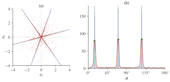
Sparsity is the assumption that makes overcomplete separation practical. At a time point where only source $j$ is active, $\bx(t) = s_j(t)\,\ba_j$ lies on the line through $\ba_j$. If such single-source points are common, the scatter plot of the data consists of $n$ lines through the origin, and their directions estimate the columns of $\bA$ up to scale and sign. Sparse component analysis (SCA) estimates $\bA$ by clustering the directions of the data points and then recovers the sources by $\ell_1$ minimization or a related sparse method.

稀疏性是使过完备分离切实可行的假设。在只有源 $j$ 活跃的时刻，$\bx(t) = s_j(t)\,\ba_j$ 落在过 $\ba_j$ 的直线上。如果这样的单源点很常见，数据的散点图就由 $n$ 条过原点的直线组成，这些直线的方向在尺度和符号意义下估计了 $\bA$ 的各列。稀疏成分分析（SCA）通过对数据点的方向聚类来估计 $\bA$，再用 $\ell_1$ 最小化或相关的稀疏方法恢复源。

The script below does this for three sparse sources and two sensors. Each source is Laplace-distributed but active only 20% of the time, so that about 38% of the samples have exactly one active source and 10% have two or more. The columns are estimated from the peaks of a smoothed histogram of the directions of the larger data points, and the sources by the shortest-path rule of Section 12.3第 12.3 节.

下面的脚本对两个传感器上的三个稀疏源完成这一过程。每个源服从拉普拉斯分布，但只在 20% 的时间里活跃，因此约 38% 的样本恰有一个活跃源，10% 的样本有两个或更多。各列由较大数据点的方向的平滑直方图的峰值来估计，源则用Section 12.3第 12.3 节中的最短路径法则恢复。

import numpy as np

rng = np.random.default_rng(0)
n, T = 3, 4000
S = rng.laplace(size=(n, T))
S *= rng.random((n, T)) < 0.2                 # each source active 20% of time
theta = np.deg2rad([15.0, 70.0, 125.0])       # true column directions
A = np.vstack([np.cos(theta), np.sin(theta)]) # 2 x 3, unit-norm columns
X = A @ S + 0.01 * rng.normal(size=(2, T))    # two sensors, weak noise

# 1) columns: peaks of the histogram of directions of the larger points
keep = np.linalg.norm(X, axis=0) > 0.2
ang = np.arctan2(X[1, keep], X[0, keep]) % np.pi   # sign removed
width = np.pi / 180
h, edges = np.histogram(ang, bins=180, range=(0, np.pi))
h = np.convolve(np.r_[h[-2:], h, h[:2]], np.ones(5) / 5, "valid")  # circular
peaks = [i for i in range(180)
         if h[i] >= h[i - 1] and h[i] > h[(i + 1) % 180]]
top = sorted(peaks, key=lambda i: -h[i])[:n]
th_hat = np.sort(edges[top] + width / 2)
A_hat = np.vstack([np.cos(th_hat), np.sin(th_hat)])
print("estimated angles (deg):", np.round(np.rad2deg(th_hat), 1))

# 2) sources: the l1 solution uses the two signed columns adjacent to x(t)
dirs = np.r_[th_hat, th_hat + np.pi]          # the 2n signed directions
S_l1 = np.zeros((n, T))
for t in range(T):
    rel = (dirs - np.arctan2(X[1, t], X[0, t])) % (2 * np.pi)
    i, j = np.argmin(rel) % n, np.argmax(rel) % n   # one on each side
    S_l1[[i, j], t] = np.linalg.solve(A_hat[:, [i, j]], X[:, t])
S_pinv = np.linalg.pinv(A_hat) @ X            # minimum l2-norm solution

def snr_db(S_est):
    err = np.sum((S - S_est) ** 2, axis=1)
    return np.round(10 * np.log10(np.sum(S ** 2, axis=1) / err), 1)
print("SNR (dB), l1:  ", snr_db(S_l1))
print("SNR (dB), pinv:", snr_db(S_pinv))

The script prints

脚本输出

estimated angles (deg): [ 14.5  70.5 125.5]
SNR (dB), l1:   [10.7  9.  10.8]
SNR (dB), pinv: [5.1 3.5 5.3]

The three directions are found to within half a degree, half the 1° bin width of the histogram. The $\ell_1$ estimates of the sources have signal-to-noise ratios of 9 to 11 dB, against 3.5 to 5.3 dB for the minimum-norm solution. The remaining error comes mainly from the time points with two or more active sources, for which the two-column explanation chosen by $\ell_1$ is wrong, exactly as in Example 12.4例 12.4. Figure 12.1图 12.1 shows the data and the histogram.

三个方向的估计误差都在半度以内，即直方图 1° 箱宽的一半。源的 $\ell_1$ 估计的信噪比为 9 到 11 dB，而最小范数解只有 3.5 到 5.3 dB。剩余误差主要来自有两个或更多活跃源的时刻：在这些时刻，$\ell_1$ 选出的双列解释是错的，正如Example 12.4例 12.4所示。Figure 12.1图 12.1画出了数据与直方图。

Most real signals are not sparse in time, but become sparse after a linear transform such as the short-time Fourier transform (STFT) or a wavelet transform. Because the transform is linear and is applied to each sensor separately, an instantaneous mixture keeps its form in the transform domain, $\tilde\bx = \bA\tilde\bs$, where the coefficients are far sparser. Bofill and Zibulevsky (2001) estimated $\bA$ for two sensors from the angular distribution of the transformed data and recovered the sources by the shortest-path rule in the transform domain. DUET (Jourjine, Rickard & Yılmaz, 2000) treats two microphones that receive each source with its own attenuation and delay. It assumes W-disjoint orthogonality: in every time–frequency bin at most one source is active. The ratio of the two STFTs in a bin then gives the relative attenuation and delay of the dominant source, a two-dimensional histogram of these parameters has one peak per source, and each source is recovered by keeping the bins assigned to its peak (binary time–frequency masking).

大多数真实信号在时域上并不稀疏，但经过短时 Fourier 变换（STFT）或小波变换之类的线性变换之后会变得稀疏。由于变换是线性的，并且对每个传感器分别作用，瞬时混合在变换域中保持原来的形式 $\tilde\bx = \bA\tilde\bs$，而其中的系数要稀疏得多。Bofill 和 Zibulevsky（2001）对两个传感器的情形，由变换后数据的角度分布估计 $\bA$，再在变换域中用最短路径法则恢复源。DUET（Jourjine, Rickard & Yılmaz, 2000）处理的是两只麦克风以各自的衰减和延迟接收每个源的情形。它假设 W 不相交正交性：每个时频单元中至多有一个源活跃。于是一个时频单元中两路 STFT 之比给出主导源的相对衰减与延迟，这两个参数的二维直方图对每个源有一个峰，把分配给某个峰的时频单元保留下来（二值时频掩蔽），就恢复出相应的源。

The single-source assumption can be relaxed. Georgiev, Theis and Cichocki (2005) showed that if every sample has at most $m - 1$ active sources, the data lie on a union of hyperplanes, each spanned by $m - 1$ columns of $\bA$, and gave conditions (columns in general position and enough samples on each hyperplane) under which clustering the data into hyperplanes identifies $\bA$ up to permutation and scaling and allows the sources to be recovered. Learning can also be done by likelihood. Lewicki and Sejnowski (2000) maximized an approximation of $p(\bx \mid \bA) = \int p(\bx \mid \bA, \bs)\,p(\bs)\,d\bs$ obtained by Laplace's method around the MAP estimate of the sources, with Laplacian priors; they showed that overcomplete bases can approximate the distribution of natural data better than complete ones, and the same machinery separates more sources than mixtures. The model is closely related to the sparse coding of natural images by Olshausen and Field (1997).

单源假设可以放宽。Georgiev、Theis 和 Cichocki（2005）指出，若每个样本至多有 $m - 1$ 个活跃源，数据就落在若干超平面的并集上，每个超平面由 $\bA$ 的 $m - 1$ 列张成；他们给出了一些条件（各列处于一般位置，且每个超平面上有足够多的样本），在这些条件下把数据聚类到各超平面就能在置换和尺度意义下辨识 $\bA$，并恢复出源。学习也可以基于似然进行。Lewicki 和 Sejnowski（2000）采用拉普拉斯先验，在源的 MAP 估计附近用 Laplace 方法近似 $p(\bx \mid \bA) = \int p(\bx \mid \bA, \bs)\,p(\bs)\,d\bs$，并最大化这一近似；他们表明过完备基能比完备基更好地逼近自然数据的分布，同一套方法还能分离多于混合个数的源。这一模型与 Olshausen 和 Field（1997）对自然图像的稀疏编码密切相关。

12.6 Why the overcomplete case is harder为什么过完备情形更难

Identifiability holds, but estimation is harder than in the square case for four reasons.

可辨识性依然成立，但估计比方阵情形更难，原因有四。

• No whitening shortcut. In the square case second-order statistics reduce the unknown to a rotation with $n(n-1)/2$ parameters. With $n > m$ the covariance $\bA\bA^\top$ fixes only $m(m+1)/2$ numbers, whitening cannot make $n$ columns orthogonal, and what remains is not a rotation to be searched for.
• Higher-order statistics. The columns are determined by statistics beyond the covariance, and the larger $n/m$, the higher the order needed (Section 12.4第 12.4 节). Sample cumulants of high order have large variance and are sensitive to outliers (Section 5.6第 5.6 节), so many more samples are required.
• No closed-form likelihood. The likelihood $p(\bx \mid \bA)$ is an integral of $\prod_i p_i(s_i)$ over the $(n - m)$-dimensional solution set of Proposition 12.3命题 12.3 (or over $\R^n$ when there is noise), with no closed form for non-Gaussian priors. It has to be approximated, by Laplace's method, by sampling, or by expectation–maximization schemes, and the resulting likelihood surfaces tend to be flat, with many local optima.
• Irreducible recovery error. Even with $\bA$ known exactly, the sources are recovered only approximately, with an error governed by how sparse they are (Fact 12.5事实 12.5).

• 没有白化这条捷径。在方阵情形下，二阶统计量把未知量化归为一个有 $n(n-1)/2$ 个参数的旋转。当 $n > m$ 时，协方差 $\bA\bA^\top$ 只确定 $m(m+1)/2$ 个数，白化无法使 $n$ 个列两两正交，剩下的也不是一个可供搜索的旋转。
• 需要高阶统计量。各列由协方差之外的统计量确定，而 $n/m$ 越大，所需的阶数越高（Section 12.4第 12.4 节）。高阶样本累积量方差大，对离群值敏感（Section 5.6第 5.6 节），因此需要多得多的样本。
• 似然没有闭式。似然 $p(\bx \mid \bA)$ 是 $\prod_i p_i(s_i)$ 在Proposition 12.3命题 12.3的 $n - m$ 维解集上（有噪声时在 $\R^n$ 上）的积分，对非高斯先验没有闭式。它只能近似计算，例如用 Laplace 方法、抽样或期望最大化类的方法，而所得的似然曲面往往很平坦，局部最优也多。
• 恢复误差无法消除。即使 $\bA$ 完全已知，源也只能近似恢复，误差取决于源有多稀疏（Fact 12.5事实 12.5）。

Sparsity helps at every step: it creates single-source points that reveal $\bA$, makes $\ell_1$ recovery accurate, and concentrates the likelihood around the true columns. Without it, overcomplete ICA remains possible in principle but is statistically demanding.

稀疏性在每一步都有帮助：它产生揭示 $\bA$ 的单源点，使 $\ell_1$ 恢复准确，并使似然集中在真实的列附近。没有稀疏性，过完备 ICA 在原理上仍然可行，但在统计上要求很高。

12.7 Exercises习题