Part V · Chapter 13第五部分 · 第 13 章
Nonlinear ICA非线性 ICA
Why general nonlinear ICA is not identifiable, and how temporal structure or auxiliary variables restore identifiability (TCL, PCL, iVAE).
为什么一般的非线性 ICA 不可辨识,以及时间结构或辅助变量如何恢复可辨识性(TCL、PCL、iVAE)。
13.1 Nonlinear mixing非线性混合
The linear model is an idealization. Sensors saturate, images are formed through occlusion, shading and perspective, and the factors that generate natural data are rarely added together with fixed weights. The natural generalization keeps independent sources but replaces the matrix by a function:
线性模型 是一种理想化。传感器会饱和;图像经由遮挡、明暗与透视而形成;生成自然数据的各种因素,也很少以固定的权重简单相加。最自然的推广是保留相互独立的源,而把矩阵换成一个函数:
where is an unknown invertible function, the mixing function. We assume as many observations as sources and, where needed, that and are smooth. Nonlinear ICA seeks a function such that the components of recover the sources. With this is ordinary ICA, which Chapter 4第 4 章 showed to be solvable up to scaling and permutation whenever at most one source is Gaussian.
其中 是未知的可逆函数,称为混合函数。我们假设观测维数与源的个数相同,并在需要时假设 与 都是光滑的。非线性 ICA 要找一个函数 ,使 的各分量恢复出源。当 时,这就是普通的 ICA;Chapter 4第 4 章已经证明,只要至多一个源是高斯的,它就能在尺度与置换的意义下求解。
Some ambiguity is unavoidable, and it is larger than in the linear case. Let be a permutation of and invertible scalar functions, and set . Each is a function of a different source, so the are again independent. Write for the invertible map ; then with . The data cannot tell from , so the best one can hope for is the following.
某种不确定性是无法避免的,而且比线性情形更大。设 是 的一个置换, 是可逆的标量函数,令 。每个 只是某一个源的函数,且所涉及的源各不相同,因此 仍然相互独立。记 为可逆映射 ,则 ,其中 。数据无法区分 与 ,所以最理想的结果也只能是下面这种意义下的分离。
Definition 13.1 (separation and identifiability)定义 13.1(分离与可辨识性)
A function separates the sources of the model (13.1) if there are a permutation and invertible scalar functions such that for every . Nonlinear ICA is identifiable within a class of models if, for every model in the class, every invertible whose outputs are independent separates the sources.
若存在置换 与可逆标量函数 ,使得对每个 都有 ,则称函数 分离了模型 (13.1) 的源。若在某一类模型中,对其中每个模型,每个使输出相互独立的可逆函数 都能分离源,则称非线性 ICA 在这一类模型中可辨识。
Two features of this definition matter later. First, the marginal distributions of the sources carry no information. With the cumulative distribution function (CDF) of and the standard Gaussian CDF, the map turns any source with a continuous, strictly increasing CDF into a standard Gaussian variable (Exercise 13.1习题 13.1). Non-Gaussianity of the marginals, the basis of linear ICA, is therefore useless here. Second, since one may as well assume Gaussian sources, the rotational ambiguity of Gaussian vectors from Section 1.4第 1.4 节 is never far away. The next section turns this observation into a theorem.
这个定义有两点后面会用到。第一,源的边缘分布不携带任何信息。记 为 的累积分布函数(CDF), 为标准高斯分布的 CDF,则映射 能把任何 CDF 连续且严格递增的源变成标准高斯变量(Exercise 13.1习题 13.1)。线性 ICA 赖以成立的边缘非高斯性,在这里毫无用处。第二,既然不妨假设源都是高斯的,Section 1.4第 1.4 节中高斯向量的旋转不确定性便近在眼前。下一节把这一观察变成定理。
13.2 Independence is not enough仅有独立性是不够的
The basic tool is the probability integral transform: if a random variable has a continuous CDF , then is uniform on . Applying it one coordinate at a time, each time conditionally on the coordinates already processed, turns any random vector into one with independent uniform components. Write for the conditional CDF of given , and define
基本工具是概率积分变换:若随机变量 的 CDF 是连续的,则 在 上均匀分布。逐个坐标地使用这一变换,每次都以已经处理过的坐标为条件,就能把任何随机向量变成分量独立且均匀分布的向量。记 为给定 时 的条件 CDF,定义
where is the CDF of . This triangular map is often called the Darmois construction; Hyvärinen and Pajunen (1999) used it to show that nonlinear ICA always has solutions, and far too many of them. It is a nonlinear counterpart of Gram–Schmidt orthogonalization: the -th output keeps only what adds to the coordinates before it, and for a Gaussian vector the construction reduces to Cholesky whitening followed by (Exercise 13.2习题 13.2).
其中 是 的 CDF。这个三角形映射通常称为 Darmois 构造;Hyvärinen 与 Pajunen(1999)用它证明了非线性 ICA 总是有解,而且解多得过了头。它相当于 Gram–Schmidt 正交化的非线性版本:第 个输出只保留 相对于前面各坐标新增的部分;对高斯向量而言,这一构造就退化为 Cholesky 白化再接上 (Exercise 13.2习题 13.2)。
Theorem 13.2 (non-identifiability of nonlinear ICA)定理 13.2(非线性 ICA 的不可辨识性)
(a) Let be a random vector in whose density is positive on an open convex set and zero outside it. Then the map of (13.2) is a bijection from onto , and is uniformly distributed on . In particular are independent.
(a) 设随机向量 的密度在某个开凸集 上处处为正、在其外为零。则 (13.2) 定义的映射 是从 到 的双射,且 在 上均匀分布。特别地, 相互独立。
(b) Let and let be independent, each with a CDF that is continuous and strictly increasing on an open interval carrying all of its probability. Then there is an invertible map such that has the same distribution as , so that its components are independent, while its first component is strictly increasing in and strictly decreasing in . Consequently, for every invertible mixing function , the map produces independent outputs without separating the sources, and nonlinear ICA is not identifiable.
(b) 设 , 相互独立,且每个 的 CDF 在某个承载其全部概率的开区间上连续且严格递增。则存在可逆映射 ,使 与 同分布(因而其分量相互独立),而它的第一个分量关于 严格递增、关于 严格递减。于是,对任何可逆混合函数 ,映射 的输出相互独立,却并没有分离源:非线性 ICA 不可辨识。
Proof.证明
(a) Let be the projection of onto the first coordinates, an open convex set, and let be the marginal density of ; it is positive on , because it integrates the density over a nonempty open set of the remaining coordinates. For fixed , the values of with form an open interval, on which the conditional density is positive. So the conditional CDF of , as a function of , increases continuously and strictly from 0 to 1 across this interval, and every has exactly one preimage . Solving for in turn shows that is a bijection from onto .
(a) 记 为 在前 个坐标上的投影,它是开凸集;记 为 的边缘密度。由于它是把密度在其余坐标的一个非空开集上积分得到的,所以在 上为正。固定 ,使 的 构成一个开区间,条件密度 在这个区间上为正。因此 的条件 CDF 作为 的函数,在该区间上从 0 连续且严格地增加到 1,每个 恰有一个原像 。依次对 求解 ,即知 是从 到 的双射。
Now fix and condition on . Given these values, has a continuous distribution with CDF , so by the probability integral transform is uniform on whatever the conditioning values are. Its conditional distribution does not depend on , so is independent of , and hence of , which is a function of these coordinates. Therefore, for all ,
再固定 ,以 为条件。给定这些值, 服从 CDF 为 的连续分布,由概率积分变换,无论条件取什么值, 都在 上均匀分布。它的条件分布与 无关,所以 与 独立,从而与作为这些坐标之函数的 独立。于是对任意 ,
and by induction the joint CDF of is , that of the uniform distribution on .
归纳可得 的联合 CDF 为 ,即 上均匀分布的 CDF。
(b) Let be the CDF of . By the probability integral transform, is standard Gaussian, so . Let rotate the first two coordinates by the angle and leave the others unchanged; then as well (Exercise 1.3习题 1.3). Set , with the inverse of on its interval. The components of are independent because those of are, and the -th has CDF , so has the distribution of . The map is a composition of bijections, hence invertible. Finally , so is strictly increasing in , hence in , and strictly decreasing in , hence in . Since , the outputs of are independent, yet is not a function of any single source.
(b) 记 为 的 CDF。由概率积分变换, 服从标准高斯分布,所以 。令 把前两个坐标旋转 角、其余坐标不变,则同样有 (Exercise 1.3习题 1.3)。令 ,其中 是 在其区间上的反函数。由于 的分量相互独立, 的分量也相互独立,且第 个分量的 CDF 为 ,所以 与 同分布。 是若干双射的复合,因而可逆。最后,,所以 关于 严格递增,从而关于 严格递增;关于 严格递减,从而关于 严格递减。由于 , 的输出相互独立,但 不是任何单个源的函数。
Part (a) applies to any random vector, mixture or not. Independent outputs therefore cannot certify that a nonlinear unmixing has found the sources, even when the mixing happens to be linear.
(a) 部分适用于任何随机向量,不论它是否来自混合。因此,即使混合恰好是线性的,输出相互独立也不能证明一个非线性解混找到了源。
Example 13.3 (the Darmois construction on a linear mixture)例 13.3(对线性混合做 Darmois 构造)
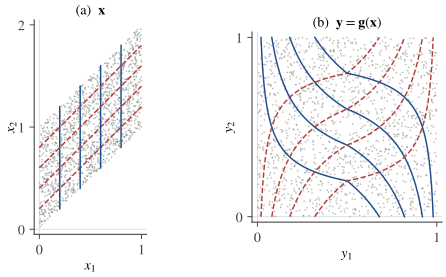
Let be independent and uniform on , and observe the linear mixture , , which linear ICA would separate. Apply the Darmois construction taking first. The sum of two independent uniforms has the triangular CDF for and for , and given , the variable is uniform on . Hence
设 相互独立,都在 上均匀分布,观测到线性混合 ,;线性 ICA 可以把它分开。现在先取 、再取 做 Darmois 构造。两个独立均匀变量之和服从三角分布,其 CDF 为: 时 , 时 ;而给定 时, 在 上均匀分布。因此
The support of is an open parallelogram, so by part (a) of Theorem 13.2定理 13.2, with the coordinates taken in the order , the outputs and are independent and uniform. Yet each depends on both sources.
的支撑集是一个开平行四边形,所以按 的坐标次序应用Theorem 13.2定理 13.2的 (a) 部分,输出 与 相互独立且均匀分布。但每个输出都同时依赖两个源。
The following script checks both claims on samples.
下面的脚本在 个样本上检验这两点。
import numpy as np
from scipy import stats

rng = np.random.default_rng(1)
T = 100_000
s1 = rng.uniform(0, 1, T)                 # two independent sources
s2 = rng.uniform(0, 1, T)
x1, x2 = s1, s1 + s2                      # a linear mixture

# Darmois construction, taking x2 first and x1 second
y1 = np.where(x2 <= 1, x2**2 / 2, 1 - (2 - x2)**2 / 2)   # CDF of x2 (triangular)
lo, hi = np.maximum(0, x2 - 1), np.minimum(1, x2)         # given x2, x1 ~ U(lo, hi)
y2 = (x1 - lo) / (hi - lo)                                # conditional CDF of x1

# Test that (y1, y2) is uniform on the unit square: chi-square on a 10 x 10 grid
H, _, _ = np.histogram2d(y1, y2, bins=10, range=[[0, 1], [0, 1]])
chi2 = ((H - T / 100) ** 2 / (T / 100)).sum()
print(f"chi2 = {chi2:.1f} on 99 df, p = {stats.chi2.sf(chi2, 99):.2f}")
# ... yet each output depends on both sources
print(np.round(np.corrcoef([y1, y2, s1, s2])[:2, 2:], 2))
It prints on 99 degrees of freedom (; over repeated seeds the -values spread evenly over , as they should under independence) and the correlations of with , : both outputs depend strongly on both sources. In Figure 13.1图 13.1, lines of constant and of constant , straight in the plane, become curves in the square.
脚本输出 (自由度 99,;换用不同的随机种子重复, 值均匀地散布在 上,与独立性相符),以及 与 的相关系数 :两个输出都与两个源强相关。在Figure 13.1图 13.1 中, 平面里的 等值线与 等值线都是直线,到了 正方形中却成了曲线。
Part (b) of the theorem rests on a symmetry: a map that sends a distribution with independent components onto itself while mixing the coordinates. Rotations of are the simplest such maps, but there are many more. Let denote the rotation of the plane by the angle and define
定理的 (b) 部分依赖于一种对称性:存在把分量独立的分布映到自身、同时又把坐标混在一起的映射。 的旋转是这类映射中最简单的,但远不止于此。记 为平面上转角为 的旋转,定义
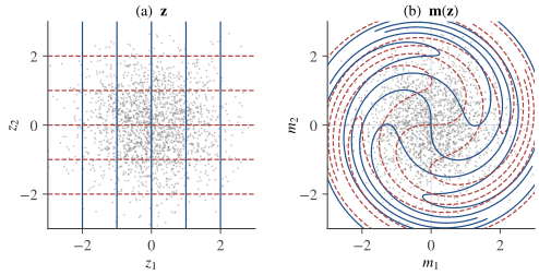
which turns each circle centered at the origin by an angle proportional to its squared radius. If , then (Exercise 13.3习题 13.3): its components are independent standard Gaussians, although each depends on both and in a complicated way (Figure 13.2图 13.2). The map is smooth with a smooth inverse, so requiring to be smooth does not remove the ambiguity. Composed with the componentwise maps and their inverses, as in the proof of part (b), such measure-preserving maps produce a continuum of spurious solutions, which are smooth when and are smooth and the source densities are smooth and positive on their intervals. Without further information, independence of the outputs says almost nothing about whether they are the sources.
它把每个以原点为圆心的圆旋转一个与半径平方成正比的角度。若 ,则 (Exercise 13.3习题 13.3):它的两个分量是相互独立的标准高斯变量,但每个分量都以复杂的方式同时依赖 与 (Figure 13.2图 13.2)。这个映射光滑且逆映射也光滑,所以要求 光滑并不能消除不确定性。像 (b) 部分的证明那样,把这类保测映射与逐分量映射 及其逆复合起来,就得到一整族连续变化的伪解;当 与 光滑、源密度光滑且在各自区间上为正时,这些伪解也是光滑的。没有其他信息时,输出相互独立几乎不能说明它们是不是源。
13.3 Restricting the mixing function限制混合函数
Theorem 13.2定理 13.2 leaves two ways forward: restrict the class of mixing functions, or give the sources more structure than independence. The oldest restriction is the post-nonlinear (PNL) model of Taleb and Jutten (1999), in which a linear mixture passes through an invertible nonlinearity in each sensor,
Theorem 13.2定理 13.2留下了两条出路:限制混合函数的类别,或者赋予源比独立性更多的结构。最早的限制是 Taleb 与 Jutten(1999)提出的后非线性(post-nonlinear, PNL)模型:线性混合在每个传感器中再经过一个可逆的非线性变换,
as happens when sensors respond nonlinearly, for instance by saturating. The separating structure mirrors the model: first a scalar nonlinearity in each channel, then a matrix, , where applies to the -th coordinate. If every composition is affine, what remains is a linear ICA problem. Taleb and Jutten (1999) showed that, under conditions on , the sources and the nonlinearities, independence of the outputs forces exactly this: each is affine and is a scaled permutation, so the sources are recovered up to the usual scaling, permutation and additive constants. The conditions have been weakened in later work, and we do not state them precisely here.
传感器响应非线性(例如饱和)时就是这种情形。分离结构与模型相对应:先在每个通道上作用一个标量非线性函数 ,再乘以一个矩阵,即 ,其中 把 作用于第 个坐标。如果每个复合函数 都是仿射的,剩下的就是一个线性 ICA 问题。Taleb 与 Jutten(1999)证明,在关于 、源和非线性函数的一定条件下,输出相互独立恰好迫使这一点成立:每个 都是仿射的,且 是带尺度的置换矩阵,于是源可以在通常的尺度、置换以及加性常数的意义下恢复。后来的工作放宽了这些条件,这里不再精确陈述。
The PNL model (13.3) escapes Theorem 13.2定理 13.2 because its separating structure, scalar functions and one matrix, is too rigid to reproduce maps that act jointly on several coordinates, such as the Darmois map or the spiral of Figure 13.2图 13.2. Restricting to conformal maps has a similar effect: Hyvärinen and Pajunen (1999) gave a uniqueness result in two dimensions, and Buchholz, Besserve and Schölkopf (2022) extended such results to higher dimensions, in each case up to a small group of simple transformations. The price is generality, since the processes behind images or neural recordings are neither post-nonlinear nor conformal. The rest of the chapter keeps arbitrary and adds structure to the sources instead.
PNL 模型 (13.3) 之所以能躲开Theorem 13.2定理 13.2,是因为它的分离结构( 个标量函数加一个矩阵)过于刚性,无法复现同时作用于多个坐标的映射,例如 Darmois 映射或Figure 13.2图 13.2 中的螺旋映射。把 限制为共形映射也有类似效果:Hyvärinen 与 Pajunen(1999)给出了二维情形的唯一性结果,Buchholz、Besserve 与 Schölkopf(2022)把这类结果推广到更高维,两者都是在一个由简单变换构成的小群的意义下唯一。代价是一般性:图像或神经记录背后的生成过程既不是后非线性的,也不是共形的。本章其余部分对 不加限制,转而给源增加结构。
13.4 Temporal structure: time-contrastive and permutation-contrastive learning时间结构:时间对比学习与置换对比学习
For linear ICA, temporal structure was an alternative to non-Gaussianity (Chapter 9第 9 章). For nonlinear ICA it becomes a source of identifiability in its own right. The methods of Hyvärinen and Morioka turn estimation into classification, using a simple fact about logistic regression. Suppose a classifier is trained on equal numbers of samples from two densities and and models the posterior probability of the first class as . The true posterior is , so the optimal regression function is the log-density ratio
对线性 ICA 而言,时间结构是非高斯性之外的另一种选择(Chapter 9第 9 章)。对非线性 ICA 而言,它本身就成了可辨识性的来源。Hyvärinen 与 Morioka 的方法把估计问题变成分类问题,所依据的是逻辑回归的一个简单事实。设用来自两个密度 与 的等量样本训练一个分类器,它把第一类的后验概率建模为 。真实后验是 ,所以最优的回归函数就是对数密度比
With flexible models and enough data, logistic regression therefore learns a log-density ratio; this is the principle of noise-contrastive estimation (Gutmann & Hyvärinen, 2012). In nonlinear ICA the two densities share the same mixing function, and their ratio turns out to be blind to it.
因此,只要模型足够灵活、数据足够多,逻辑回归学到的就是对数密度比;这正是噪声对比估计的原理(Gutmann & Hyvärinen, 2012)。在非线性 ICA 中,两个密度共享同一个混合函数,而它们的比值恰好对这个混合函数“视而不见”。
Time-contrastive learning时间对比学习
Suppose the sources are nonstationary. The time series is divided into segments ; within each segment the sources are independent, and their log-densities change from segment to segment through an exponential family,
假设源是非平稳的。把时间序列分成 共 段;在每一段内各源相互独立,而它们的对数密度通过一个指数族随段而变:
where and are fixed functions, is a modulation parameter and a normalizing constant. With and , for instance, is the inverse variance of source in segment : the sources are Gaussian with power that fluctuates over time. Time-contrastive learning (TCL; Hyvärinen & Morioka, 2016) trains a multinomial logistic regression to predict the segment label from the observation,
其中 与 是固定的函数, 是调制参数, 是归一化常数。例如取 ,,则 就是源 在第 段内方差的倒数:源是高斯的,但功率随时间起伏。时间对比学习(time-contrastive learning, TCL;Hyvärinen & Morioka, 2016)训练一个多项逻辑回归,从观测预测它所在的段:
where is a feature extractor, in practice a neural network, trained jointly with the weights and biases .
其中 是特征提取器,实践中是一个神经网络,与权重 和偏置 一起训练。
Proposition 13.4 (time-contrastive learning)命题 13.4(时间对比学习)
Assume that with invertible and both and differentiable; that within each segment the sources are independent with log-densities (13.4), no being almost surely constant; and that the matrix with entries has rank . If the classifier (13.5) equals the true posterior , then there are an invertible matrix and a vector such that
设 ,其中 可逆,且 与 均可微;在每一段内各源相互独立,对数密度为 (13.4),且没有哪个 几乎必然为常数; 矩阵 (元素为 )的秩为 。若分类器 (13.5) 等于真实后验 ,则存在可逆的 矩阵 与向量 ,使得
Proof.证明
Let be the proportion of samples in segment . By Bayes' rule , so equating the log-odds of segment against segment 1 under the classifier and under the truth gives
记 为第 段样本所占的比例。由 Bayes 公式,,所以令分类器与真实后验中第 段相对第 1 段的对数几率相等,得到
By the change-of-variables formula, with and denoting a Jacobian matrix,
由变量替换公式,记 , 表示 Jacobian 矩阵,则
The Jacobian term is the same in every segment and cancels from the difference of log-densities, and so do the ; by (13.4),
Jacobian 项在各段中都相同,在对数密度之差中被消去, 也一样;由 (13.4),
Stacking the equations for gives , where has rows and collects the constants. Because has full column rank, its pseudo-inverse satisfies , and multiplying by gives the claim with and . Finally, if were singular, some vector would satisfy , and would be almost surely constant within a segment. That is impossible: for an index with , would then almost surely equal a function of the other components, which are independent of it, and a random variable independent of itself is almost surely constant. Hence is invertible.
把 的方程堆叠起来,得到 ,其中 的各行为 , 汇集了各常数项。由于 列满秩,其伪逆满足 ,左乘 即得结论,其中 ,。最后,若 奇异,则存在向量 使 ,于是在一段之内 几乎必然为常数。这不可能:取 的下标 ,则 几乎必然等于其余分量的某个函数,而其余分量与它独立;与自身独立的随机变量几乎必然为常数,矛盾。故 可逆。
This is a slight generalization of Theorem 1 of Hyvärinen and Morioka (2016), with the same proof. The cancellation of the Jacobian is the heart of the matter: in the likelihood of a single segment, is an unknown function that can absorb almost anything, but a ratio of two densities generated by the same mixing function does not contain it. The rank condition on is a sufficient variability requirement: at least segments, with source distributions that change in sufficiently different ways (Exercise 13.4习题 13.4). It remains to undo . The are independent within each segment, but generally not when the segments are pooled, because the pooled density is a mixture of product densities. The natural last step is therefore a linear method that uses the nonstationarity: within segment the covariance matrix of equals times a diagonal matrix times , so joint diagonalization of the segment-wise covariance matrices recovers the (Chapter 9第 9 章), provided no two of them have proportional variance profiles across segments. An ordinary ICA of the pooled features is exact only when the pooled are independent and non-Gaussian. Note that need not be an invertible function of : with the sign of is lost.
这是 Hyvärinen 与 Morioka(2016)定理 1 的一个小推广,证明完全相同。Jacobian 被消去是问题的关键:在单独一段的似然中, 是一个几乎什么都能吸收的未知函数,而由同一混合函数生成的两个密度之比根本不含这一项。关于 的秩条件是一种充分变化性要求:至少要有 段,而且各源分布的变化方式要足够不同(Exercise 13.4习题 13.4)。剩下的是去掉 。各 在每一段内相互独立,但把各段合并后一般并不独立,因为合并后的密度是若干乘积密度的混合。因此最后一步宜采用利用非平稳性的线性方法:在第 段内, 的协方差矩阵等于 乘一个对角矩阵再乘 ,所以只要没有两个 的方差随段变化的轮廓成比例,对各段协方差矩阵做联合对角化就能恢复各 (Chapter 9第 9 章)。只有当合并后的 相互独立且非高斯时,对合并数据做普通 ICA 才是精确的。注意 未必是 的可逆函数:当 时, 的符号就丢失了。
Permutation-contrastive learning置换对比学习
Permutation-contrastive learning (PCL; Hyvärinen & Morioka, 2017) assumes instead that the sources are stationary with temporal dependence. It discriminates pairs of consecutive observations from pairs with a randomly chosen time , which have the same marginals but no temporal dependence. Its regression function is a sum of terms , each depending only on one learned feature at the two time points. Hyvärinen and Morioka proved that the learned recover the sources up to permutation and componentwise invertible transformations if is a bijection that is twice differentiable with a twice differentiable inverse, the sources are mutually independent, stationary and ergodic processes, and each source is
置换对比学习(permutation-contrastive learning, PCL;Hyvärinen & Morioka, 2017)则假设源是平稳的、但在时间上相互依赖。它区分相邻时刻的观测对 与随机选取时刻 构成的观测对 ;后者的边缘分布相同,但没有时间依赖。它的回归函数是若干项 之和,每一项只依赖于一个学到的特征 在两个时刻的取值。Hyvärinen 与 Morioka 证明:若 是二阶可微且逆映射也二阶可微的双射,各源是相互独立的平稳遍历过程,并且每个源都满足下面两个条件,则学到的 能在置换与逐分量可逆变换的意义下恢复源:
- Uniformly dependent: writing for the joint density of and , the cross-derivative exists, is continuous and is nonzero everywhere.
- Not quasi-Gaussian: this cross-derivative is not of the form for a constant and a function .
- 一致依赖:记 为 与 的联合密度,交叉导数 存在、连续且处处非零。
- 非拟高斯:这个交叉导数不能写成 的形式,其中 为常数, 为某个函数。
A stationary Gaussian autoregressive process has a constant cross-derivative and is therefore quasi-Gaussian. For quasi-Gaussian sources PCL recovers only an invertible linear mixture of transformed sources, which a further linear step must unmix (Hyvärinen & Morioka, 2017).
平稳的高斯自回归过程的交叉导数是常数,因而是拟高斯的。对拟高斯的源,PCL 只能恢复变换后各源的一个可逆线性混合,还需要再做一步线性解混(Hyvärinen & Morioka, 2017)。
13.5 Auxiliary variables and generalized contrastive learning辅助变量与广义对比学习
TCL and PCL share a structure. In both, an observed variable, the segment label in TCL and the past observation in PCL, changes the distribution of the sources without changing the mixing function. Hyvärinen, Sasaki and Turner (2019) made this the definition of the model: the sources are conditionally independent given an observed auxiliary variable ,
TCL 与 PCL 有共同的结构。两者都有一个观测到的变量(TCL 中是段标号 ,PCL 中是前一时刻的观测 ),它改变源的分布,却不改变混合函数。Hyvärinen、Sasaki 与 Turner(2019)把这一点直接作为模型的定义:给定一个观测到的辅助变量 ,各源条件独立,
where does not depend on . The auxiliary variable can be a time index or segment label, a past observation, a class label, a stimulus, or a simultaneously recorded second modality. The sources need not be marginally independent. Estimation is by generalized contrastive learning (GCL): a logistic regression discriminates true pairs from pairs in which is drawn independently of , for instance by shuffling the observed values of , using a regression function of the form
其中 与 无关。辅助变量可以是时间标号或段标号、过去的观测、类别标签、刺激,或者同时记录的另一种模态。各源不必边缘独立。估计方法是广义对比学习(generalized contrastive learning, GCL):用逻辑回归区分真实的配对 与配对 ,其中 的抽取与 独立(例如把观测到的 值随机打乱),回归函数取如下形式:
By the principle of Section 13.4第 13.4 节, the optimal regression function is
由Section 13.4第 13.4 节中的原理,最优的回归函数是
To state the identifiability result, write and for the first and second derivatives of with respect to , and collect their values at in a vector of length :
为了陈述可辨识性结果,用 、 表示 关于 的一阶与二阶导数,并把它们在 处的值排成一个长度为 的向量:
Theorem 13.5 (identifiability with an auxiliary variable; Hyvärinen, Sasaki & Turner, 2019)定理 13.5(辅助变量下的可辨识性;Hyvärinen, Sasaki & Turner, 2019)
Assume that
假设
- the data follow (13.6), with invertible and both and twice continuously differentiable;
- each is twice continuously differentiable in for every ;
- (sufficient variability) for every there are values of the auxiliary variable such that the vectors , , are linearly independent;
- the logistic regression with regression function (13.7) attains its optimum in the limit of infinite data, where the and are flexible enough to represent it and is constrained to be invertible and twice continuously differentiable with a twice continuously differentiable inverse.
- 数据服从 (13.6),其中 可逆,且 与 均二阶连续可微;
- 对每个 , 关于 二阶连续可微;
- (充分变化性)对每个 ,存在辅助变量的 个取值 ,使 个向量 ()线性无关;
- 回归函数为 (13.7) 的逻辑回归在无穷数据的极限下达到最优,其中 与 足够灵活,能够表示最优解,并且 被约束为可逆、二阶连续可微、逆映射也二阶连续可微。
Then there are a permutation and invertible scalar functions such that for every : the features separate the sources in the sense of Definition 13.1定义 13.1.
则存在置换 与可逆标量函数 ,使得对每个 都有 :这些特征按Definition 13.1定义 13.1的意义分离了源。
Proof.证明
Write and , so that and is a twice continuously differentiable bijection of . By the change-of-variables formula, and equal and , respectively, plus the same term , where is the marginal density of the sources. This term cancels in the optimal regression function, so that, as functions of and for every ,
记 ,,于是 ,且 是 上二阶连续可微的双射。由变量替换公式, 与 分别等于 与 再加上同一项 ,其中 是源的边缘密度。这一项在最优回归函数中相互抵消,因此作为 的函数,对每个 都有
Subtract this identity at a second value , and write for the difference between the values at and at . The last term cancels, and
用另一个取值 处的恒等式去减它,并用 表示在 处与在 处的取值之差。最后一项被消去,得到
By assumptions 1, 2 and 4, the right side is twice continuously differentiable in . The left side is a sum of functions of one coordinate each; since it is differentiable, so is each term, and its partial derivative with respect to depends on alone. Hence its mixed partial derivatives with respect to and , , vanish, and so do those of the right side. Computing the latter with the chain rule, and writing for and for the vector with entries and , gives
由假设 1、2、4,右边关于 二阶连续可微。左边是若干单坐标函数之和;既然它可微,每一项也可微,而且它对 的偏导数只依赖于 。因此它对 与 ()的混合偏导数为零,右边的混合偏导数也就为零。用链式法则计算右边的混合偏导数,记 为 ,并记 为分量是 与 的向量,得到
This holds for every and every pair , ; no smoothness of or of the was needed. Fix , let , and take the values of assumption 3 for this . With the identity says that is orthogonal to linearly independent vectors, so . In particular for all and all : each row of the Jacobian matrix has at most one nonzero entry. As is invertible, it has exactly one nonzero entry in each row and each column, and by continuity the position of these entries is the same for every (Exercise 13.6习题 13.6). Hence each is a strictly monotonic function of a single coordinate , for a permutation ; inverting, is an invertible function of the single source , which is the claim with .
这对每个 以及每一对 、 都成立;整个推导不需要 或 的任何光滑性。固定 ,令 ,并对这个 取假设 3 中的 。令 ,上式说明 与 个线性无关的向量都正交,所以 。特别地,对所有 与所有 有 :Jacobian 矩阵 的每一行至多有一个非零元。由于 可逆,它每行每列恰有一个非零元,而且由连续性,这些非零元的位置对所有 都相同(Exercise 13.6习题 13.6)。因此存在置换 ,使每个 都是单个坐标 的严格单调函数;反过来, 是单个源 的可逆函数,取 即为所证。
The theorem places no restriction on . Its price is assumption 3: at every point, must act on the source distributions in at least sufficiently different ways. This fails when each conditional log-density is an exponential family with a single sufficient statistic, as in (13.4) with replaced by : every difference is then a combination of the same vectors (Hyvärinen, Sasaki & Turner, 2019; Exercise 13.5习题 13.5). This is the situation of TCL, which is why Proposition 13.4命题 13.4 identified the sufficient statistics only up to a linear transformation. With two or more sufficient statistics per source, modulated in sufficiently independent ways, the assumption holds except in degenerate cases. TCL and PCL are special cases of GCL with and .
这个定理对 没有任何限制,代价是假设 3:在每一点, 都必须以至少 种足够不同的方式作用于源的分布。若每个条件对数密度都是只有一个充分统计量的指数族,即把 (13.4) 中的 换成 ,这一点就不成立:此时每个差向量 都是同样 个向量的线性组合(Hyvärinen, Sasaki & Turner, 2019;Exercise 13.5习题 13.5)。这正是 TCL 的情形,也解释了为什么Proposition 13.4命题 13.4只能在线性变换的意义下辨识充分统计量。若每个源有两个或更多充分统计量,且它们以足够独立的方式被调制,则除退化情形外该假设都成立。TCL 与 PCL 是 GCL 在 与 时的特例。
13.6 Identifiable variational autoencoders可辨识的变分自编码器
Contrastive methods learn the demixing but neither the mixing function nor the source densities, and they assume noiseless data. Khemakhem, Kingma, Monti and Hyvärinen (2020) placed the auxiliary-variable model inside a latent-variable model that can be fitted by maximum likelihood. In the identifiable VAE (iVAE), the observation is a noisy function of the sources, , where with , is injective and the noise is independent of . Given , the sources are independent with exponential-family densities
对比学习方法学到的是解混函数 ,既不学混合函数,也不学源的密度,而且假设数据没有噪声。Khemakhem、Kingma、Monti 与 Hyvärinen(2020)把辅助变量模型放进一个可以用最大似然拟合的隐变量模型中。在可辨识变分自编码器(identifiable VAE, iVAE)中,观测是源的带噪函数 ,其中 ,, 是单射,噪声 与 独立。给定 ,各源相互独立,且服从指数族密度
Here is a base measure, a normalizing constant, the are sufficient statistics and the their natural parameters; stack them as and . Sources that are Gaussian given , with means and variances that depend on , are the case with and .
其中 是基测度, 是归一化常数, 是充分统计量, 是相应的自然参数;把它们分别排成 与 。给定 时为高斯分布、均值与方差都随 变化的源,对应于 ,,。
Theorem 13.6 (Khemakhem et al., 2020)定理 13.6(Khemakhem et al., 2020)
Let two parameter values and of this model give the same conditional distribution of given , for every . Assume that
设该模型的两组参数 与 对每个 都给出相同的条件分布 。假设
- the set of points where the characteristic function of the noise density vanishes has measure zero;
- is injective;
- each is differentiable almost everywhere, and for each the functions are linearly independent on every set of positive measure;
- (sufficient variability) there are values of the auxiliary variable such that the matrix with columns , , is invertible.
- 噪声密度的特征函数取零值的点集测度为零;
- 是单射;
- 每个 几乎处处可微,且对每个 ,函数 在任何正测度集上线性无关;
- (充分变化性)存在辅助变量的 个取值 ,使以 ()为列的 矩阵 可逆。
Then there are an invertible matrix and a vector such that, for all in the image of ,
则存在可逆的 矩阵 与向量 ,使得对 值域中的所有 都有
We omit the proof. Its core is the argument of Proposition 13.4命题 13.4, applied after the noise has been removed by deconvolution, which assumption 1 permits: subtracting the log-densities at cancels the Jacobians and the base measures, and is inverted. The same paper shows that is a block permutation matrix if , the are twice differentiable and has all second-order cross-derivatives, and a scaled permutation if , the are not monotonic and the partial derivatives of are continuous. The sufficient statistics of each estimated source are then an affine function of those of a single true source, which for injective is separation in the sense of Definition 13.1定义 13.1. The extra conditions matter. With , and Gaussian base measures, the sources given are , and is of the same form for every orthogonal , with means : the sources are identified only up to a rotation.
这里略去证明。其核心就是Proposition 13.4命题 13.4的论证,只是先要借助假设 1 用反卷积去掉噪声:减去 处的对数密度,消去 Jacobian 与基测度,再对 求逆。同一篇论文还证明:若 , 二阶可微,且 的所有二阶交叉偏导数存在,则 是分块置换矩阵;若 , 不单调,且 的各偏导数连续,则 是带尺度的置换矩阵。此时每个估计源的充分统计量都是某一个真实源的充分统计量的仿射函数;当 为单射时,这就是Definition 13.1定义 13.1意义下的分离。这些附加条件并非可有可无。取 ,,基测度为高斯,则给定 时源服从 ;对任何正交矩阵 , 也具有同样的形式,均值为 :源只能辨识到一个旋转。
The iVAE fits the model as a variational autoencoder (Kingma & Welling, 2014). A decoder represents , the prior is (13.8) with computed by a neural network, and an encoder approximates the posterior. Training maximizes the evidence lower bound
iVAE 以变分自编码器(Kingma & Welling, 2014)的形式拟合这个模型。解码器表示 ,先验为 (13.8),其中 由神经网络计算,编码器 近似后验。训练时最大化证据下界
whose gap is the KL divergence from to the true posterior. If the encoder family contains the true posterior, maximizing the bound with infinite data recovers the parameters up to the equivalence of Theorem 13.6定理 13.6 (Khemakhem et al., 2020). An ordinary VAE, by contrast, has the unconditional prior , which rotations and measure-preserving maps such as of Figure 13.2图 13.2 leave invariant. Composing the decoder with such a map leaves the likelihood unchanged, so an ordinary VAE cannot be identifiable; a prior that changes with breaks the symmetry.
两者之差就是 相对真实后验的 KL 散度。若编码器族包含真实后验,则在无穷数据下最大化这个下界,能在Theorem 13.6定理 13.6的等价意义下恢复参数(Khemakhem et al., 2020)。相比之下,普通 VAE 的先验是与条件无关的 ,旋转以及像Figure 13.2图 13.2 中 那样的保测映射都使它保持不变。把解码器与这样的映射复合,似然不变,所以普通 VAE 不可能可辨识;而随 变化的先验打破了这种对称性。
13.7 Disentanglement and its limits解耦表示及其局限
Deep representation learning often aims for disentangled representations, in which each coordinate captures one independent factor of variation, such as pose, lighting or identity in images of faces. If the factors are independent and the data are a deterministic invertible function of them, this is exactly nonlinear ICA, and the results of this chapter apply. Locatello et al. (2019) proved that for every factorized density on with there is an infinite family of bijections such that has the distribution of and every partial derivative is nonzero almost everywhere: maps like the spiral of Figure 13.2图 13.2, which entangle every output with every factor while leaving the distribution unchanged. They concluded that unsupervised learning of disentangled representations is impossible without inductive biases on both the models and the data. A large experimental study in the same paper, with more than 12,000 trained models on seven data sets, found that well-disentangled models could not be identified reliably without supervision, and that results depended substantially on random seeds and hyperparameters.
深度表示学习常常追求解耦的表示,即每个坐标只刻画一个独立的变化因素,例如人脸图像中的姿态、光照或身份。如果各因素相互独立,而数据是它们的确定性可逆函数,这就恰好是非线性 ICA,本章的结论都适用。Locatello 等(2019)证明:对 ()上任何可分解的密度,都存在无穷多个双射 ,使 与 同分布,且每个偏导数 几乎处处非零。这正是Figure 13.2图 13.2 中螺旋那样的映射:它让每个输出与每个因素都纠缠在一起,分布却保持不变。他们由此得出结论:若对模型和数据都没有归纳偏置,无监督地学习解耦表示是不可能的。同一篇论文中的大规模实验训练了 12,000 多个模型、涉及七个数据集,发现没有监督就无法可靠地挑出解耦良好的模型,而且结果在相当程度上取决于随机种子与超参数。
Nonlinear ICA theory says which inductive biases suffice: an observed auxiliary variable that modulates the sources (TCL, PCL, GCL, iVAE), or a restricted class of mixing functions (post-nonlinear, conformal). The guarantees have limits. They are asymptotic, assuming infinite data, flexible enough function classes and a global optimum; assumptions such as conditional independence given or sufficient variability can rarely be verified from data; and the sources are recovered only up to permutation and componentwise invertible transformations, so their scale, units and sometimes their sign are lost. Hyvärinen, Khemakhem and Morioka (2023) review the field and its connections to self-supervised learning.
非线性 ICA 理论回答了哪些归纳偏置是足够的:一个调制源分布的观测辅助变量(TCL、PCL、GCL、iVAE),或者一个受限的混合函数类(后非线性或共形映射)。这些保证都有局限。它们是渐近结论,假设数据无穷多、函数类足够灵活、优化达到全局最优;给定 的条件独立、充分变化性之类的假设,很少能从数据中检验;而且源只能在置换与逐分量可逆变换的意义下恢复,其尺度、单位乃至符号都可能丢失。Hyvärinen、Khemakhem 与 Morioka(2023)综述了这一领域及其与自监督学习的联系。
Key points
本章要点
- Nonlinear ICA models with an invertible . At best the sources are recovered up to permutation and componentwise invertible transformations, so the shape of their marginal distributions carries no information.
- Without further assumptions the problem is not identifiable: the Darmois construction makes any random vector independent, and measure-preserving maps of yield a continuum of spurious solutions for sources with continuous, strictly increasing CDFs, smooth ones when the source densities are smooth and positive.
- Restricting the mixing function, as in post-nonlinear mixtures, restores identifiability at the cost of generality.
- An observed auxiliary variable that modulates the source distributions makes a log-density ratio free of the unknown Jacobian; contrastive learning then recovers the sources under a sufficient-variability condition (TCL, PCL, GCL).
- The iVAE gives comparable guarantees within a likelihood framework with noise; a VAE with an unconditional Gaussian prior is not identifiable.
- The impossibility result for unsupervised disentanglement is the same non-identifiability; auxiliary variables and restricted mixing functions are inductive biases that resolve it.
- 非线性 ICA 的模型是 ,其中 可逆。最好的结果也只是在置换与逐分量可逆变换的意义下恢复源,因此源的边缘分布形状不携带任何信息。
- 不加其他假设时问题不可辨识:Darmois 构造能把任何随机向量变得独立, 的保测映射对 CDF 连续且严格递增的源都能给出一整族伪解;当源密度光滑且为正时,这些伪解也是光滑的。
- 限制混合函数(例如后非线性混合)可以恢复可辨识性,代价是失去一般性。
- 若有一个调制源分布的观测辅助变量,对数密度比就不再含未知的 Jacobian;在充分变化性条件下,对比学习能够恢复源(TCL、PCL、GCL)。
- iVAE 在带噪声的似然框架中给出类似的保证;先验为与条件无关的高斯分布的 VAE 不可辨识。
- 无监督解耦表示学习的不可能性结论,本质上就是同一种不可辨识性;辅助变量与受限的混合函数都是能消除它的归纳偏置。
13.8 Exercises习题
Exercise 13.1习题 13.1 basic基础
Let be independent, a permutation and invertible scalar functions. (a) Show that , , are independent. (b) Let have a CDF that is continuous and strictly increasing on an open interval carrying all its probability. Show that . What does this imply for the role of non-Gaussianity in nonlinear ICA?
设 相互独立, 是一个置换, 是可逆标量函数。(a) 证明 ()相互独立。(b) 设 的 CDF 在某个承载其全部概率的开区间上连续且严格递增,证明 。这对非高斯性在非线性 ICA 中的作用意味着什么?
Show solution查看解答
(a) For any sets , the event equals . Since is a permutation, these events concern different sources, so by independence
(a) 对任意集合 ,事件 等于 。由于 是置换,这 个事件涉及 个不同的源,由独立性得
(b) Let be the inverse of on its interval. For and ,
(b) 记 为 在其区间上的反函数。对 与 ,
so is uniform on and is standard Gaussian. Combining (a) and (b), any model (13.1) with such sources can be rewritten, with the mixing function , as a model with independent standard Gaussian sources. The shape of the marginals therefore says nothing about which directions are the sources; in contrast to linear ICA, non-Gaussianity cannot be what identifies them, and the information must come from restrictions on or from additional structure such as an auxiliary variable.
所以 在 上均匀分布, 服从标准高斯分布。结合 (a) 与 (b),任何具有这类源的模型 (13.1) 都可以改写为混合函数为 、源为独立标准高斯变量的模型。因此边缘分布的形状完全不能说明哪些方向是源;与线性 ICA 不同,非高斯性不可能用来辨识源,所需的信息只能来自对 的限制,或者来自辅助变量之类的额外结构。
Exercise 13.2习题 13.2 intermediate进阶
(a) Let be Gaussian with zero mean, unit variances and correlation , . Compute the Darmois construction (13.2) explicitly and verify directly that and are independent. (b) For a zero-mean Gaussian with nonsingular covariance , lower triangular with positive diagonal (Cholesky factor), show that the construction gives with . (c) Let with and invertible. When is each a function of a single source?
(a) 设 是零均值、单位方差、相关系数为 ()的高斯向量。显式写出 Darmois 构造 (13.2),并直接验证 与 独立。(b) 设 是零均值高斯向量,协方差 非奇异,其中 是对角元为正的下三角矩阵(Cholesky 因子)。证明该构造给出 ,其中 。(c) 设 ,, 可逆。什么时候每个 都只是单个源的函数?
Show solution查看解答
(a) , so . Given , , so with . The variables and are jointly Gaussian with unit variances, and , so they are independent; and are functions of one each. (b) Since with lower triangular, , where are functions of (and conversely), and is independent of them because . Hence, given , is Gaussian with mean and standard deviation , and its conditional CDF evaluated at is . Part (a) is the case . (c) Now and , where is orthogonal because . Each is a function of a single source exactly when every row of has a single nonzero entry, that is, when is a signed permutation, or equivalently when is lower triangular up to permuting and changing the signs of its columns. For a generic this fails: the construction returns independent outputs that are a rotation of the sources, which is precisely the Gaussian ambiguity of Section 1.4第 1.4 节.
(a) ,所以 。给定 ,,所以 ,其中 。变量 与 联合高斯、方差均为 1,且 ,因此相互独立;而 、 各自只是其中一个的函数。(b) 由于 且 为下三角,,其中 是 的函数(反之亦然),而由于 , 与它们独立。因此给定 , 服从均值为 、标准差为 的高斯分布,它的条件 CDF 在 处的值为 。(a) 正是 的情形。(c) 此时 ,,其中 是正交矩阵,因为 。每个 都只是单个源的函数,当且仅当 的每一行只有一个非零元,即 是带符号的置换矩阵;等价地, 在对列作置换和变号之后是下三角矩阵。对一般的 这并不成立:构造给出的独立输出是源的一个旋转,这正是Section 1.4第 1.4 节中高斯情形的不确定性。
Exercise 13.3习题 13.3 intermediate进阶
Let and with . (a) Show that . (b) Show that is an infinitely differentiable bijection of with an infinitely differentiable inverse. (c) Conclude that for two independent standard Gaussian sources and any smooth invertible mixing , some smooth invertible produces independent outputs without separating the sources.
设 ,,。(a) 证明 。(b) 证明 是 上无穷次可微的双射,且逆映射也无穷次可微。(c) 由此说明:对于两个独立的标准高斯源和任何光滑可逆的混合 ,都存在光滑可逆的 ,其输出相互独立却没有分离源。
Show solution查看解答
(a) Write . For , the radius and the angle are independent and is uniform on , because the density does not depend on . The map sends to . Given , the shifted angle is again uniform on , whatever the shift, so it is independent of and uniform; the pair (radius, angle) of therefore has the same joint law as that of , and so does . (b) The components of are
(a) 记 。对 ,由于密度 与 无关,半径 与角度 相互独立,且 在 上均匀分布。该映射把 变为 。给定 ,无论平移多少,平移后的角度在 上仍均匀分布,因而与 独立且均匀;所以 的(半径,角度)与 的有相同的联合分布, 与 也就同分布。(b) 的分量为
compositions of polynomials with and , hence infinitely differentiable. A rotation preserves norms, so , and the map , infinitely differentiable for the same reason, inverts . (With the angle instead, the map would fail to be twice differentiable at the origin.) (c) Let , smooth and invertible with inverse . Then has independent standard Gaussian components by (a). But equals when , which varies with , and equals when , which varies with ; so is a function of neither source alone, and does not separate.
它们是多项式与 、 的复合,因而无穷次可微。旋转保持范数,所以 ,而映射 (同理无穷次可微)就是 的逆。(若转角取 ,映射在原点处就不是二阶可微的。)(c) 令 ,它光滑可逆,逆为 。由 (a), 的分量是独立的标准高斯变量。但 在 时等于 ,随 变化;在 时等于 ,随 变化。所以 不是任何单个源的函数, 没有分离源。
Exercise 13.4习题 13.4 basic基础
In Proposition 13.4命题 13.4: (a) why must there be at least segments? (b) Suppose all sources are modulated in lockstep, for constants and a function . Show that the rank condition fails for , however many segments there are. (c) Give a modulation with segments that satisfies it.
关于Proposition 13.4命题 13.4:(a) 为什么段数至少要有 ?(b) 设各源同步调制,即 ,其中 为常数、 为某个函数。证明当 时,无论段数多少,秩条件都不成立。(c) 给出一个只有 段且满足秩条件的调制方式。
Show solution查看解答
(a) has rows, and its rank cannot exceed its number of rows, so rank requires . (b) , so with and , a matrix of rank at most 1. Intuitively, segments then differ only in overall loudness, which says nothing about how the loudness is shared among the sources. (c) Let for all , and in segment (for ) let only source change, , for . Then , which has rank . With this means that each source in turn has its variance halved while the others stay at variance 1.
(a) 有 行,秩不超过行数,所以秩为 要求 。(b) ,所以 ,其中 ,,这个矩阵的秩至多为 1。直观地说,此时各段之间只有整体响度的差别,无法说明响度在各源之间如何分配。(c) 令所有 都有 ;在第 段()只让源 变化:, 时 。则 ,秩为 。取 时,这相当于让各源轮流把方差减半,而其他源的方差保持为 1。
Exercise 13.5习题 13.5 advanced硬核
(a) Let the sources be independent given with . Compute and show that assumption 3 of Theorem 13.5定理 13.5 fails at every . (b) Now let . Exhibit values of for which the assumption holds at every .
(a) 设给定 时各源独立,且 。计算 ,并证明Theorem 13.5定理 13.5的假设 3 在每个 处都不成立。(b) 现设 。给出 的 组取值,使该假设在每个 处都成立。
Show solution查看解答
(a) With ,
(a) 记 ,则
so and . Hence, with the standard basis of ,
所以 ,。于是,记 为 的标准基,有
and every difference lies in the span of the vectors . At most of the differences can be linearly independent, whatever the values . (b) With , now and . Take the baseline with all , . For , let differ from the baseline only in : the difference is . For , let differ from the baseline only in (variance ): the difference is . These differences are linearly independent for every . In a vanishing linear combination with coefficients for the first kind and for the second, coordinate equals , so all , and then all . Modulating the means as well as the variances supplies the missing directions.
并且每个差向量 都落在 个向量 张成的子空间中。无论 如何取, 个差向量中至多只有 个线性无关。(b) 仍记 ,此时 ,。取基准 :所有 ,。对 ,令 与基准只差在 ,对应的差向量为 ;再令 与基准只差在 (方差为 ),对应的差向量为 。对每个 ,这 个差向量都线性无关:在一个为零的线性组合中,记第一类向量的系数为 、第二类的为 ,则第 个坐标等于 ,所以所有 ,进而所有 。同时调制均值与方差,补上了所缺的 个方向。
Exercise 13.6习题 13.6 advanced硬核
Complete the last step of the proof of Theorem 13.5定理 13.5. Let be a continuously differentiable bijection whose Jacobian matrix is invertible for every and has at most one nonzero entry in each row. Show that there are a permutation and strictly monotonic functions such that for all and .
补全Theorem 13.5定理 13.5证明的最后一步。设 是连续可微的双射,其 Jacobian 矩阵 对每个 都可逆,且每行至多有一个非零元。证明存在置换 与严格单调函数 ,使对所有 与 都有 。
Show solution查看解答
Fix . An invertible matrix has no zero row, so each row has exactly one nonzero entry, say in column . If two rows had their nonzero entries in the same column, some other column would be zero and the matrix singular; so is a permutation. Next, the entries are continuous. At a given , the entries are nonzero, so they remain nonzero on a neighborhood of ; since each row has only one nonzero entry, on that neighborhood. The map is therefore locally constant on the connected set , hence constant; call it . Then everywhere for , so by the mean value theorem does not change when any coordinate other than changes, and for a function of one variable. Its derivative is continuous and never zero, so by the intermediate value theorem it has a constant sign, and is strictly monotonic.
固定 。可逆矩阵没有零行,所以每行恰有一个非零元,设其位于第 列。若有两行的非零元位于同一列,则另有某一列全为零,矩阵奇异;所以 是一个置换。其次,各元素 连续。在给定的 处, 个元素 非零,因而在 的某个邻域内保持非零;由于每行只有一个非零元,在该邻域内 。于是 在连通集 上局部恒定,从而恒定,记为 。这样当 时处处有 ,由中值定理,改变 以外的任何坐标都不会改变 ,所以 ,其中 是一元函数。它的导数 连续且处处非零,由介值定理其符号恒定,故 严格单调。
13.9 References参考文献
- Buchholz, S., Besserve, M., & Schölkopf, B. (2022). Function classes for identifiable nonlinear independent component analysis. In Advances in Neural Information Processing Systems 35 (pp. 16946–16961).
- Gutmann, M. U., & Hyvärinen, A. (2012). Noise-contrastive estimation of unnormalized statistical models, with applications to natural image statistics. Journal of Machine Learning Research, 13, 307–361.
- Hyvärinen, A., Khemakhem, I., & Morioka, H. (2023). Nonlinear independent component analysis for principled disentanglement in unsupervised deep learning. Patterns, 4(10), 100844.
- Hyvärinen, A., & Morioka, H. (2016). Unsupervised feature extraction by time-contrastive learning and nonlinear ICA. In Advances in Neural Information Processing Systems 29 (pp. 3765–3773).
- Hyvärinen, A., & Morioka, H. (2017). Nonlinear ICA of temporally dependent stationary sources. In Proceedings of the 20th International Conference on Artificial Intelligence and Statistics (PMLR 54, pp. 460–469).
- Hyvärinen, A., & Pajunen, P. (1999). Nonlinear independent component analysis: Existence and uniqueness results. Neural Networks, 12(3), 429–439.
- Hyvärinen, A., Sasaki, H., & Turner, R. E. (2019). Nonlinear ICA using auxiliary variables and generalized contrastive learning. In Proceedings of the 22nd International Conference on Artificial Intelligence and Statistics (PMLR 89, pp. 859–868).
- Khemakhem, I., Kingma, D. P., Monti, R. P., & Hyvärinen, A. (2020). Variational autoencoders and nonlinear ICA: A unifying framework. In Proceedings of the 23rd International Conference on Artificial Intelligence and Statistics (PMLR 108, pp. 2207–2217).
- Kingma, D. P., & Welling, M. (2014). Auto-encoding variational Bayes. In International Conference on Learning Representations.
- Locatello, F., Bauer, S., Lucic, M., Rätsch, G., Gelly, S., Schölkopf, B., & Bachem, O. (2019). Challenging common assumptions in the unsupervised learning of disentangled representations. In Proceedings of the 36th International Conference on Machine Learning (PMLR 97, pp. 4114–4124).
- Taleb, A., & Jutten, C. (1999). Source separation in post-nonlinear mixtures. IEEE Transactions on Signal Processing, 47(10), 2807–2820.