Natural Gradient, Infomax and Stability自然梯度、Infomax 与稳定性

7.1 From a contrast to an update rule从对比函数到更新规则

Chapter 6第 6 章 reduced ICA to an optimization problem: find the unmixing matrix $\bW$ that maximizes the log-likelihood (6.1), or equivalently minimizes the mutual information of the outputs. This chapter turns that problem into algorithms that adjust $\bW$ step by step. Three questions run through it. In which direction should $\bW$ move? How does the behaviour of the algorithm depend on the unknown mixing matrix $\bA$? And which solutions are attractors, so that the algorithm actually settles on them?

Chapter 6第 6 章把 ICA 归结为一个优化问题：寻找使对数似然 (6.1) 最大的解混矩阵 $\bW$，或者等价地，使输出的互信息最小。本章把这个问题变成逐步调整 $\bW$ 的算法。贯穿全章的有三个问题：$\bW$ 应当沿什么方向移动？算法的行为如何依赖于未知的混合矩阵 $\bA$？哪些解是吸引子，也就是说，算法实际会停在哪些解上？

The answers are, in order: along the relative or natural gradient, which needs no matrix inversion; not at all, a property called equivariance; and the separating solutions attract the algorithm when a simple condition linking the nonlinearity to the source distributions holds, and not when it fails. The same condition explains why the original Infomax algorithm separates typical super-Gaussian sources such as speech but fails on some sub-Gaussian ones, and how the extended version repairs this.

三个答案依次是：沿着相对梯度（即自然梯度）的方向移动，这一方向不需要矩阵求逆；完全不依赖，这一性质称为等变性；当非线性函数与源分布之间满足一个简单的条件时，分离解吸引算法，条件不满足时则不然。同一个条件解释了为什么原始的 Infomax 算法能分离语音这类常见的超高斯源，却在某些亚高斯源上失效，以及扩展 Infomax 如何弥补这一缺陷。

Throughout the chapter the model is square ($m = n$, after the PCA reduction of Section 3.6第 3.6 节 if necessary), $\bA$ is invertible, and the sources are independent with zero mean. The algorithms use model densities $p_i$ that need not be the true ones. Their scores $\varphi_i = -p_i'/p_i$ are the nonlinearities of the algorithm, collected in $\bphi(\by) = (\varphi_1(y_1), \dots, \varphi_n(y_n))^\top$. When the model is right, $\varphi_i$ is the true score $\psi_i$ of Definition 6.1定义 6.1.

本章始终假设模型是方阵情形（$m = n$，必要时先做Section 3.6第 3.6 节的 PCA 降维），$\bA$ 可逆，各源相互独立且均值为零。算法使用的是模型密度 $p_i$，它不必是真实密度。模型密度的得分函数 $\varphi_i = -p_i'/p_i$ 就是算法中的非线性函数，记作向量 $\bphi(\by) = (\varphi_1(y_1), \dots, \varphi_n(y_n))^\top$。模型正确时，$\varphi_i$ 就是Definition 6.1定义 6.1中的真实得分函数 $\psi_i$。

7.2 The ordinary gradient普通梯度

For one observation, the log-likelihood of $\bW$ is $\sum_i \log p_i(\bw_i^\top\bx) + \log|\det\bW|$, where $\bw_i^\top$ is the $i$-th row of $\bW$. Its expectation

对单个观测，$\bW$ 的对数似然为 $\sum_i \log p_i(\bw_i^\top\bx) + \log|\det\bW|$，其中 $\bw_i^\top$ 是 $\bW$ 的第 $i$ 行。它的期望

is the objective of this chapter. Batch algorithms replace $\E$ by the sample average $\hat\E$ over $\bx(1), \dots, \bx(T)$, which turns $\ell$ into $\frac1T\log L(\bW)$. Since $\partial\log|\det\bW|/\partial\bW = \bW^{-\top}$ (Section A.6第 A.6 节) and $\partial\log p_i(\bw_i^\top\bx)/\partial\bw_i = -\varphi_i(y_i)\,\bx$, the gradient is

就是本章的目标函数。批量算法把 $\E$ 换成对 $\bx(1), \dots, \bx(T)$ 的样本平均 $\hat\E$，此时 $\ell$ 就是 $\frac1T\log L(\bW)$。由 $\partial\log|\det\bW|/\partial\bW = \bW^{-\top}$（Section A.6第 A.6 节）以及 $\partial\log p_i(\bw_i^\top\bx)/\partial\bw_i = -\varphi_i(y_i)\,\bx$，梯度为

Setting the gradient to zero and multiplying on the right by $\bW^\top$ gives the estimating equations $\E[\bphi(\by)\by^\top] = \bI$, that is, $\E[\varphi_i(y_i)\,y_j] = \delta_{ij}$ for all $i, j$. Every separating matrix satisfies the off-diagonal equations, whatever the nonlinearities: if $y_i$ and $y_j$ are multiples of two different sources, then $\E[\varphi_i(y_i)y_j] = \E[\varphi_i(y_i)]\,\E[y_j] = 0$ by independence and zero means. The diagonal equations only fix the scale of each output. This is the robustness to a wrong source model noted in Chapter 6第 6 章: the model does not move the separating points. What it decides is whether an algorithm converges to them, the subject of Section 7.5第 7.5 节.

令梯度为零并右乘 $\bW^\top$，得到估计方程 $\E[\bphi(\by)\by^\top] = \bI$，即对所有 $i, j$ 有 $\E[\varphi_i(y_i)\,y_j] = \delta_{ij}$。无论非线性函数取什么，任何分离矩阵都满足其中的非对角方程：若 $y_i$ 与 $y_j$ 分别是两个不同源的倍数，则由独立性与零均值，$\E[\varphi_i(y_i)y_j] = \E[\varphi_i(y_i)]\,\E[y_j] = 0$。对角方程只确定各输出的尺度。这正是Chapter 6第 6 章中提到的对源模型设错的稳健性：模型不会移动分离点，它决定的是算法能否收敛到分离点，这是Section 7.5第 7.5 节的主题。

Plain gradient ascent, $\bW \leftarrow \bW + \mu\nabla\ell(\bW)$ with a step size $\mu > 0$, has two flaws. It needs the inverse $\bW^{-\top}$ at every step. More seriously, its behaviour depends on $\bA$. Write the update in terms of the global matrix $\bP = \bW\bA$, using $\bW^{-\top} = \bP^{-\top}\bA^\top$, $\bx^\top = \bs^\top\bA^\top$ and $\by = \bP\bs$:

普通的梯度上升 $\bW \leftarrow \bW + \mu\nabla\ell(\bW)$（步长 $\mu > 0$）有两个缺点。第一，每一步都要计算逆矩阵 $\bW^{-\top}$。第二，也是更严重的，它的行为依赖于 $\bA$。利用 $\bW^{-\top} = \bP^{-\top}\bA^\top$、$\bx^\top = \bs^\top\bA^\top$ 和 $\by = \bP\bs$，把更新改写成全局矩阵 $\bP = \bW\bA$ 的形式：

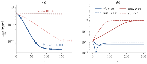
The fixed matrix $\bA^\top\bA$ acts as a preconditioner chosen by nature. When $\bA$ is ill-conditioned, the steps are long in some directions and very short in others, and no single step size suits all of them. Panel (a) of Figure 7.1图 7.1 shows the effect: with a condition number of 10, plain gradient ascent hardly moves in 150 iterations.

固定矩阵 $\bA^\top\bA$ 相当于一个由“自然”指定的预条件矩阵。$\bA$ 病态时，更新在某些方向上步子很大，在另一些方向上步子极小，没有一个统一的步长能同时适合所有方向。Figure 7.1图 7.1的（a）图显示了这一效应：条件数为 10 时，普通梯度上升在 150 次迭代中几乎原地不动。

7.3 Relative and natural gradients相对梯度与自然梯度

Cardoso and Laheld (1996) perturb $\bW$ multiplicatively, $\bW \to (\bI + \bepsilon)\bW$ with a small $n \times n$ matrix $\bepsilon$, so that the outputs change by $\by \to \by + \bepsilon\by$. To first order, $\log|\det((\bI + \bepsilon)\bW)| = \log|\det\bW| + \tr\bepsilon$ and $\log p_i\bigl(y_i + (\bepsilon\by)_i\bigr) = \log p_i(y_i) - \varphi_i(y_i)\sum_j \varepsilon_{ij}y_j$. Hence

Cardoso 与 Laheld（1996）对 $\bW$ 做乘性扰动 $\bW \to (\bI + \bepsilon)\bW$，其中 $\bepsilon$ 是一个小的 $n \times n$ 矩阵，于是输出变为 $\by \to \by + \bepsilon\by$。在一阶近似下，$\log|\det((\bI + \bepsilon)\bW)| = \log|\det\bW| + \tr\bepsilon$，且 $\log p_i\bigl(y_i + (\bepsilon\by)_i\bigr) = \log p_i(y_i) - \varphi_i(y_i)\sum_j \varepsilon_{ij}y_j$。因此

where $\langle\bB, \bepsilon\rangle = \tr(\bB^\top\bepsilon) = \sum_{ij} b_{ij}\varepsilon_{ij}$ is the Frobenius inner product. The matrix $\bI - \E[\bphi(\by)\by^\top]$ is the relative gradient; it depends on $\bW$ only through the outputs. By (7.4), among relative perturbations of a given Frobenius norm, the one that increases $\ell$ fastest is proportional to it, which gives the update

其中 $\langle\bB, \bepsilon\rangle = \tr(\bB^\top\bepsilon) = \sum_{ij} b_{ij}\varepsilon_{ij}$ 是 Frobenius 内积。矩阵 $\bI - \E[\bphi(\by)\by^\top]$ 称为相对梯度，它只通过输出依赖于 $\bW$。由 (7.4)，在 Frobenius 范数给定的所有相对扰动中，使 $\ell$ 增加最快的扰动与它成正比，由此得到更新规则

Amari, Cichocki and Yang (1996) reached the same rule as a natural gradient, a steepest-ascent direction for a geometry adapted to the problem; Amari (1998) develops the idea in general. On the group of invertible matrices, measure a small change $d\bW$ by the size of the relative change, $\|d\bW\,\bW^{-1}\|_F$. This metric is invariant under right multiplication, $\bW \to \bW\bB$, because $(d\bW\,\bB)(\bW\bB)^{-1} = d\bW\,\bW^{-1}$; right multiplication is the natural symmetry of the problem, since $\by = \bW\bx = (\bW\bB)(\bB^{-1}\bx)$. To find the steepest direction, maximize the first-order change $\langle\nabla\ell, d\bW\rangle$ subject to $\|d\bW\,\bW^{-1}\|_F = \delta$. With $d\bW = \bepsilon\bW$ the objective is $\langle\nabla\ell\,\bW^\top, \bepsilon\rangle$ under $\|\bepsilon\|_F = \delta$, maximized by $\bepsilon \propto \nabla\ell\,\bW^\top$. The steepest direction is therefore $\nabla\ell(\bW)\,\bW^\top\bW$, and by (7.2)

Amari、Cichocki 与 Yang（1996）以自然梯度的形式得到了同一规则：它是在适合本问题的几何下的最速上升方向；Amari（1998）对这一思想作了一般性的阐述。在可逆矩阵构成的群上，用相对变化的大小 $\|d\bW\,\bW^{-1}\|_F$ 来度量小变化 $d\bW$。这个度量在右乘 $\bW \to \bW\bB$ 下不变，因为 $(d\bW\,\bB)(\bW\bB)^{-1} = d\bW\,\bW^{-1}$；而右乘正是本问题的自然对称性，因为 $\by = \bW\bx = (\bW\bB)(\bB^{-1}\bx)$。为求最速方向，在约束 $\|d\bW\,\bW^{-1}\|_F = \delta$ 下最大化一阶变化量 $\langle\nabla\ell, d\bW\rangle$。令 $d\bW = \bepsilon\bW$，目标变为在 $\|\bepsilon\|_F = \delta$ 下最大化 $\langle\nabla\ell\,\bW^\top, \bepsilon\rangle$，最优解为 $\bepsilon \propto \nabla\ell\,\bW^\top$。因此最速方向是 $\nabla\ell(\bW)\,\bW^\top\bW$，再由 (7.2) 得

the direction of (7.5). It is still an ascent direction, because $\langle\nabla\ell, \nabla\ell\,\bW^\top\bW\rangle = \|\nabla\ell\,\bW^\top\|_F^2 \ge 0$, and it vanishes exactly where the ordinary gradient does. It needs no inverse. Its online form, which uses one sample at a time, is $\bW \leftarrow \bW + \mu_t\bigl(\bI - \bphi(\by(t))\,\by(t)^\top\bigr)\bW$ with $\by(t) = \bW\bx(t)$.

这正是 (7.5) 的方向。它仍是上升方向，因为 $\langle\nabla\ell, \nabla\ell\,\bW^\top\bW\rangle = \|\nabla\ell\,\bW^\top\|_F^2 \ge 0$；它为零的位置与普通梯度完全相同；并且它不需要求逆。它的在线形式每次只用一个样本：$\bW \leftarrow \bW + \mu_t\bigl(\bI - \bphi(\by(t))\,\by(t)^\top\bigr)\bW$，其中 $\by(t) = \bW\bx(t)$。

7.4 Equivariance等变性

Multiplying (7.5) on the right by $\bA$ removes the mixing matrix from the dynamics altogether.

把 (7.5) 右乘 $\bA$，混合矩阵就从动力学中完全消失了。

The algorithm sees only the sources and its current global matrix. The speed of convergence, the attained accuracy and the stability of each separating point are the same for every invertible $\bA$; they are properties of the source distributions, the nonlinearities, the step sizes and the starting point $\bP_0$. Cardoso and Laheld (1996) call algorithms with this property equivariant. (7.3) shows that plain gradient ascent is not equivariant. Figure 7.1图 7.1(a) compares the two on the same sources, started from the same $\bP_0$, for three mixing matrices with condition numbers 1, 10 and 100: the three natural-gradient curves coincide, while the ordinary gradient slows down with the conditioning.

算法“看到”的只有源和它当前的全局矩阵。收敛速度、所达到的精度以及各分离点的稳定性，对每个可逆的 $\bA$ 都一样；它们只取决于源分布、非线性函数、步长以及起点 $\bP_0$。Cardoso 与 Laheld（1996）把具有这一性质的算法称为等变算法。由 (7.3) 可见，普通梯度上升不是等变的。Figure 7.1图 7.1（a）在同一组源上、从同一个 $\bP_0$ 出发，对条件数分别为 1、10、100 的三个混合矩阵比较了两种算法：三条自然梯度曲线完全重合，而普通梯度随条件数变差而变慢。

Two caveats. Equivariance is a property of the noiseless model: with $\bx = \bA\bs + \bn$ the outputs are $\bP\bs + \bW\bn$, and the noise term depends on $\bW$ and hence on $\bA$ (Section 11.2第 11.2 节). And it says nothing about the starting point: with $\bW_0 = \bI$ the algorithm starts at $\bP_0 = \bA$, which is far from separation when $\bA$ is ill-conditioned. Whitening first starts it at the orthogonal matrix $\bP_0 = \tilde\bA$ instead, which is one good reason to whiten the data before iterating. Because performance does not depend on $\bA$, the statistical analysis of Chapter 10第 10 章 can assume $\bA = \bI$ without loss of generality.

有两点需要注意。其一，等变性只对无噪声模型成立：若 $\bx = \bA\bs + \bn$，输出为 $\bP\bs + \bW\bn$，噪声项依赖于 $\bW$，从而依赖于 $\bA$（Section 11.2第 11.2 节）。其二，等变性不涉及起点：取 $\bW_0 = \bI$ 时，算法从 $\bP_0 = \bA$ 出发，$\bA$ 病态时这个起点离分离很远。先做白化，起点就变成正交矩阵 $\bP_0 = \tilde\bA$，这是迭代之前先白化数据的一个充分理由。由于性能与 $\bA$ 无关，Chapter 10第 10 章的统计分析可以不失一般性地假设 $\bA = \bI$。

7.5 Local stability of the separating points分离点的局部稳定性

For a small step size, the batch iteration follows, and the online iteration follows on average, the ordinary differential equation $d\bW/dt = (\bI - \E[\bphi(\by)\by^\top])\bW$ obtained by letting $\mu \to 0$. By equivariance, as in (7.6), in global coordinates it reads

步长很小时，批量迭代跟随、在线迭代平均意义下跟随令 $\mu \to 0$ 得到的常微分方程 $d\bW/dt = (\bI - \E[\bphi(\by)\by^\top])\bW$。由等变性，与 (7.6) 一样，它在全局坐标下写作

Its equilibria are the solutions of the estimating equations $\E[\bphi(\by)\by^\top] = \bI$. Consider a separating one, $\bP = \bPi\bD$; after relabelling the sources, $\bPi = \bI$. The off-diagonal equations hold automatically, and the diagonal ones ask for $\E[\varphi_i(d_is_i)\,d_is_i] = 1$; we assume that this equation has a solution $d_i \ne 0$ for every $i$, as it does for all nonlinearities in this chapter. Since the sources are defined only up to scale (Proposition 1.3命题 1.3), we may replace $s_i$ by $d_is_i$. The separating point is then $\bP = \bI$, and the sources satisfy the normalization

它的平衡点就是估计方程 $\E[\bphi(\by)\by^\top] = \bI$ 的解。考虑一个分离型平衡点 $\bP = \bPi\bD$；重新给源编号后可设 $\bPi = \bI$。非对角方程自动成立，对角方程要求 $\E[\varphi_i(d_is_i)\,d_is_i] = 1$；我们假设对每个 $i$ 这个方程都有解 $d_i \ne 0$，本章出现的所有非线性函数都满足这一点。由于源只在尺度意义下确定（Proposition 1.3命题 1.3），可以用 $d_is_i$ 代替 $s_i$。这样分离点就是 $\bP = \bI$，而各源满足归一化条件

The variances $\sigma_i^2 = \E[s_i^2]$ are now set by the nonlinearities and generally differ from 1. Define

此时方差 $\sigma_i^2 = \E[s_i^2]$ 由非线性函数决定，一般不等于 1。定义

The conditions involve single sources and pairs of sources, never triples. With the normalization in force, write $\gamma_i = k_i\sigma_i^2$. Conditions (ii) and (iii) together say that $\gamma_i > 0$ and $\gamma_i\gamma_j > 1$ for all pairs. A simple sufficient condition is $\gamma_i > 1$ for every source; if two sources have $\gamma < 1$, the pair is unstable. For a Gaussian source, $\gamma_i = 1$ whatever the nonlinearity (Exercise 7.4习题 7.4), so a Gaussian source is always on the boundary; the next result shows that the true score puts every non-Gaussian source strictly inside.

这些条件只涉及单个源和源的两两组合，从不涉及三个源。在归一化条件下记 $\gamma_i = k_i\sigma_i^2$。条件（ii）与（iii）合起来就是：$\gamma_i > 0$，且对所有源对有 $\gamma_i\gamma_j > 1$。一个简单的充分条件是每个源都有 $\gamma_i > 1$；若有两个源的 $\gamma < 1$，则这一对不稳定。对高斯源，无论非线性函数取什么，都有 $\gamma_i = 1$（Exercise 7.4习题 7.4），所以高斯源总是处在边界上；下面的结果表明，用真实得分函数时，每个非高斯源都严格位于稳定区域之内。

Rescaling a variable by $c$ divides its Fisher information by $c^2$, so $\gamma_i = \sigma_i^2\,\E[\psi_i(s_i)^2]$ is the Fisher information $\mathcal{J}_i$ of the unit-variance source $s_i/\sigma_i$. The quantity that decides stability under the true model is the same one that limits the attainable accuracy in Theorem 10.10定理 10.10.

把变量乘以 $c$，其 Fisher 信息就除以 $c^2$，所以 $\gamma_i = \sigma_i^2\,\E[\psi_i(s_i)^2]$ 恰好是单位方差源 $s_i/\sigma_i$ 的 Fisher 信息 $\mathcal{J}_i$。在真实模型下决定稳定性的量，与Theorem 10.10定理 10.10中限制可达精度的量是同一个。

With a misspecified model the conditions can fail. Table 7.1表 7.1 lists $\gamma$ for three common nonlinearities, computed by numerical quadrature after solving (7.8); in every case $1 + m > 1$, so condition (i) holds. With $\varphi = \tanh$, a pair of Laplace sources is stable ($1.414^2 > 1$) but a pair of uniform sources is not ($0.762^2 \approx 0.58$). A uniform source paired with a Laplace source is still stable, since $0.762 \times 1.414 \approx 1.08$, but only barely: the smallest eigenvalue of the linearization is $0.038$, against $0.414$ for two Laplace sources, so convergence near the solution is about ten times slower. For $\varphi(y) = y^3$ one finds $\gamma = 3/(3 + \kappa)$ exactly (Exercise 7.2习题 7.2), so the cubic nonlinearity favours sub-Gaussian sources. A finite-difference Jacobian of the mean flow, computed with the same quadrature, reproduces the eigenvalues predicted by (7.9) to five decimal places in all these cases.

模型设错时，这些条件可能不成立。Table 7.1表 7.1列出了三种常用非线性函数下的 $\gamma$ 值，先解 (7.8)，再用数值积分算出；所有情形下都有 $1 + m > 1$，所以条件（i）成立。取 $\varphi = \tanh$ 时，一对拉普拉斯源是稳定的（$1.414^2 > 1$），一对均匀源则不稳定（$0.762^2 \approx 0.58$）。均匀源与拉普拉斯源配对时仍然稳定，因为 $0.762 \times 1.414 \approx 1.08$，但只是勉强稳定：线性化的最小特征值为 $0.038$，而两个拉普拉斯源时为 $0.414$，所以在解附近的收敛要慢约十倍。对 $\varphi(y) = y^3$，可以精确算出 $\gamma = 3/(3 + \kappa)$（Exercise 7.2习题 7.2），所以三次非线性偏向亚高斯源。在上述所有情形中，用同样的数值积分计算的平均流有限差分雅可比矩阵，其特征值与 (7.9) 的预测在小数点后五位一致。

The following script implements batch natural-gradient ICA and runs it from $\bW_0 = \bI$ on two uniform and on two Laplace sources, with $\varphi = \tanh$, with $\varphi(y) = y^3$, and with the extended Infomax rule of Section 7.7第 7.7 节. The printed interference is the largest ratio, over the rows of $\bP = \bW\bA$, of the second-largest to the largest entry in absolute value; it is 0 for perfect separation and near 1 for an even mixture.

下面的脚本实现了批量自然梯度 ICA，并从 $\bW_0 = \bI$ 出发，分别在两个均匀源和两个拉普拉斯源上运行，非线性函数依次取 $\varphi = \tanh$、$\varphi(y) = y^3$ 以及Section 7.7第 7.7 节的扩展 Infomax 规则。打印的干扰值是：在 $\bP = \bW\bA$ 的各行中，绝对值第二大的元素与最大元素之比的最大值；完全分离时为 0，均匀混合时接近 1。

import numpy as np

def natural_gradient_ica(X, phi, mu=0.1, iters=500):
    """Batch natural-gradient ICA: W <- W + mu (I - E[phi(y) y^T]) W."""
    n, T = X.shape
    W = np.eye(n)
    for _ in range(iters):
        Y = W @ X
        W += mu * (np.eye(n) - phi(Y) @ Y.T / T) @ W
    return W

def extended_infomax(X, mu=0.1, iters=500):
    """phi_i(y) = y + k_i tanh(y), k_i = +1 or -1 set by the switching rule."""
    n, T = X.shape
    W = np.eye(n)
    for _ in range(iters):
        Y = W @ X
        k = np.sign(np.mean(np.cosh(Y) ** -2, axis=1) * np.mean(Y ** 2, axis=1)
                    - np.mean(np.tanh(Y) * Y, axis=1))
        W += mu * (np.eye(n) - (Y + k[:, None] * np.tanh(Y)) @ Y.T / T) @ W
    return W

def interference(P):
    """Max over rows of P of second-largest / largest |entry|; 0 = separated."""
    R = np.sort(np.abs(P), axis=1)
    return np.max(R[:, -2] / R[:, -1])

rng = np.random.default_rng(0)
T = 20000
A = np.array([[1.0, 0.6],
              [0.4, 1.0]])
sources = {"uniform": rng.uniform(-np.sqrt(3), np.sqrt(3), (2, T)),   # kappa = -1.2
           "Laplace": rng.laplace(0, 1 / np.sqrt(2), (2, T))}        # kappa = +3
methods = {"tanh": lambda X: natural_gradient_ica(X, np.tanh),
           "cube": lambda X: natural_gradient_ica(X, lambda y: y ** 3),
           "extended": extended_infomax}
for sname, S in sources.items():
    for mname, method in methods.items():
        W = method(A @ S)
        print(f"{sname:8s} {mname:9s} interference = {interference(W @ A):.3f}")

The output is

输出为

uniform  tanh      interference = 0.987
uniform  cube      interference = 0.010
uniform  extended  interference = 0.012
Laplace  tanh      interference = 0.004
Laplace  cube      interference = 0.943
Laplace  extended  interference = 0.005

exactly the pattern of Table 7.1表 7.1: $\tanh$ fails on the uniform pair and $y^3$ on the Laplace pair, where they converge to points whose outputs are roughly even mixtures of the two sources, while each succeeds on the other pair. The residual interference of about 0.01 for the successful runs is estimation error from the finite sample (Chapter 10第 10 章). Figure 7.1图 7.1(b) shows the same dichotomy as a dynamical statement: started next to the separating point, the mismatched runs move away from it.

这恰好是Table 7.1表 7.1所预言的模式：$\tanh$ 在均匀源对上失败，$y^3$ 在拉普拉斯源对上失败，它们收敛到的点的输出大致是两个源的均匀混合；而各自在另一对源上都成功。成功运行中约 0.01 的残余干扰是有限样本带来的估计误差（Chapter 10第 10 章）。Figure 7.1图 7.1（b）以动力学的语言展示了同一个二分现象：从分离点附近出发，不匹配的运行会离开分离点。

7.6 InfomaxInfomax 算法

Bell and Sejnowski (1995) arrived at the same family of algorithms from a different principle. Pass the outputs $y_i = \bw_i^\top\bx$ through the logistic function $g(y) = 1/(1 + e^{-y})$ and choose $\bW$ to maximize the joint entropy of $\bu = (g(y_1), \dots, g(y_n))^\top$, the information that the bounded outputs carry about the input. Since $g$ is increasing and $\by = \bW\bx$, the change-of-variables formula and Proposition 2.13命题 2.13 give

Bell 与 Sejnowski（1995）从另一个原理出发得到了同一族算法。把输出 $y_i = \bw_i^\top\bx$ 通过 logistic 函数 $g(y) = 1/(1 + e^{-y})$，再选取 $\bW$ 使 $\bu = (g(y_1), \dots, g(y_n))^\top$ 的联合熵最大，也就是使有界输出所携带的关于输入的信息最大。由于 $g$ 单调递增且 $\by = \bW\bx$，由变量替换公式和Proposition 2.13命题 2.13得

Up to the constant $H(\bx)$ this is the objective $\ell(\bW)$ of (7.1) with model densities $p_i = g'$, the logistic density: Infomax is maximum likelihood with a logistic source model (Cardoso, 1997; Proposition 6.5命题 6.5). Since $g' = g(1 - g)$, the score of this model is $\varphi(y) = 2g(y) - 1 = \tanh(y/2)$ (Exercise 7.1习题 7.1). Bell and Sejnowski's gradient is $\nabla H(\bu) = \bW^{-\top} + \E[(\mathbf{1} - 2\mathbf{g}(\by))\bx^\top]$, where $\mathbf{1}$ is the vector of ones and $\mathbf{g}$ acts componentwise; this is (7.2) with $\bphi = 2\mathbf{g} - \mathbf{1}$. They also adapt a bias $\bw_0$ in $\by = \bW\bx + \bw_0$, which we omit for centered data. In practice the algorithm is usually run in its natural-gradient form.

除去常数 $H(\bx)$，这正是 (7.1) 中的目标函数 $\ell(\bW)$，其模型密度为 $p_i = g'$，即 logistic 密度：Infomax 就是以 logistic 分布为源模型的最大似然（Cardoso, 1997；Proposition 6.5命题 6.5）。由于 $g' = g(1 - g)$，这一模型的得分函数为 $\varphi(y) = 2g(y) - 1 = \tanh(y/2)$（Exercise 7.1习题 7.1）。Bell 与 Sejnowski 给出的梯度是 $\nabla H(\bu) = \bW^{-\top} + \E[(\mathbf{1} - 2\mathbf{g}(\by))\bx^\top]$，其中 $\mathbf{1}$ 是全 1 向量，$\mathbf{g}$ 逐分量作用；这就是取 $\bphi = 2\mathbf{g} - \mathbf{1}$ 时的 (7.2)。他们还在 $\by = \bW\bx + \bw_0$ 中自适应调整偏置 $\bw_0$；对已中心化的数据，这里略去偏置。实践中通常使用它的自然梯度形式。

The second row of Table 7.1表 7.1 describes this algorithm. Its separating points are stable for the usual super-Gaussian laws, such as the Laplace and logistic laws, consistent with the success of Infomax on speech and on many EEG and fMRI sources, which tend to be super-Gaussian. The exact criterion is $\gamma_i\gamma_j > 1$, not the sign of the kurtosis: a bimodal law with rare large values can have positive kurtosis and still $\gamma < 1$. A pair of uniform sources, with $0.846^2 \approx 0.72 < 1$, is unstable: Infomax cannot separate two sub-Gaussian sources of this kind, however long it runs.

Table 7.1表 7.1的第二行描述的正是这个算法。对拉普拉斯、logistic 这类常见的超高斯分布，它的分离点是稳定的，这与 Infomax 在语音以及许多 EEG 和 fMRI 源上的成功相符，因为这些源往往是超高斯的。准确的判据是 $\gamma_i\gamma_j > 1$，而不是峭度的符号：一个带有罕见大值的双峰分布可以峭度为正，却仍有 $\gamma < 1$。一对均匀源满足 $0.846^2 \approx 0.72 < 1$，是不稳定的：无论运行多久，Infomax 都无法分离两个这类亚高斯源。

7.7 Extended Infomax扩展 Infomax

Lee, Girolami and Sejnowski (1999) let each output choose between a super-Gaussian and a sub-Gaussian model. Their update is

Lee、Girolami 与 Sejnowski（1999）让每个输出在超高斯模型与亚高斯模型之间自行选择。他们的更新规则是

that is, $\varphi_i(y) = y + \eta_i\tanh(y)$. With $\eta_i = -1$ this is the score of the bimodal, sub-Gaussian density $\tfrac12\Ncal(1, 1) + \tfrac12\Ncal(-1, 1)$; with $\eta_i = +1$ it is the score of the super-Gaussian density proportional to $e^{-y^2/2}/\cosh y$. Lee et al. motivate this branch with the density proportional to $p_G(y)\operatorname{sech}^2 y$, where $p_G$ is the standard Gaussian density; the score of that density is $y + 2\tanh y$, and the rule they use, $y + \tanh y$, is the score of the density above. The sign is chosen by the switching rule

也就是 $\varphi_i(y) = y + \eta_i\tanh(y)$。$\eta_i = -1$ 时，它是双峰亚高斯密度 $\tfrac12\Ncal(1, 1) + \tfrac12\Ncal(-1, 1)$ 的得分函数；$\eta_i = +1$ 时，它是与 $e^{-y^2/2}/\cosh y$ 成正比的超高斯密度的得分函数。Lee 等人用正比于 $p_G(y)\operatorname{sech}^2 y$ 的密度（$p_G$ 为标准高斯密度）来说明这一分支，但该密度的得分函数是 $y + 2\tanh y$；他们实际使用的 $y + \tanh y$ 是上述密度的得分函数。符号由切换规则决定：

evaluated on the current outputs, in practice on each block or after each pass through the data. The rule is exactly the stability condition of Theorem 7.2定理 7.2 in disguise.

它在当前输出上估计，实践中在每个数据块上或每遍历一次数据后更新。这条规则其实就是Theorem 7.2定理 7.2中的稳定性条件换了个样子。