Tensor and Second-Order Methods: JADE and SOBI张量方法与二阶方法：JADE 与 SOBI

9.1 Separation by diagonalization通过对角化实现分离

After whitening, the remaining unknown is an orthogonal matrix $\tilde\bA$ ((3.2)). Suppose we can compute, from the data alone, a symmetric matrix of the form $\bM = \tilde\bA\bLambda\tilde\bA^\top$ with $\bLambda$ diagonal. This is an eigendecomposition: if the diagonal entries of $\bLambda$ are distinct, the eigenvectors of $\bM$ are the columns of $\tilde\bA$, up to sign and order, and $\bU = \tilde\bA^\top$ separates the sources. No iteration, contrast function or step size is needed. The covariance of $\bz$ is useless for this purpose, since it equals $\bI$, but two other families of statistics have exactly this structure: matrices built from fourth-order cumulants, which are informative when the sources are non-Gaussian, and lagged covariance matrices, which are informative when the sources are correlated in time.

白化之后，剩下的未知量是一个正交矩阵 $\tilde\bA$（(3.2)）。假设能单凭数据算出一个形如 $\bM = \tilde\bA\bLambda\tilde\bA^\top$ 的对称矩阵，其中 $\bLambda$ 是对角阵。这就是一个特征分解：若 $\bLambda$ 的对角元互不相同，$\bM$ 的特征向量就是 $\tilde\bA$ 的各列（相差符号和顺序），于是 $\bU = \tilde\bA^\top$ 就能分离各源。这里不需要迭代，不需要对比函数，也不需要步长。$\bz$ 的协方差对此毫无用处，因为它等于 $\bI$；但另有两族统计量恰好具有这种结构：由四阶累积量构造的矩阵（当源为非高斯时，它们携带信息），以及时滞协方差矩阵（当源在时间上相关时，它们携带信息）。

A single such matrix is fragile: two equal or nearly equal eigenvalues make its eigenvectors undetermined or badly estimated. Using many matrices at once and finding the one rotation that diagonalizes all of them, approximately, removes the fragility. This chapter develops that idea twice: with cumulant matrices it gives FOBI and JADE (Cardoso, 1989; Cardoso & Souloumiac, 1993), with lagged covariances AMUSE and SOBI (Tong et al., 1990; Belouchrani et al., 1997). The common computational tool is the Jacobi method for joint diagonalization (Cardoso & Souloumiac, 1996).

只用一个这样的矩阵是脆弱的：两个特征值相等或接近相等时，特征向量就不确定或估计得很差。同时使用许多矩阵，寻找一个能把它们全部近似对角化的旋转，就消除了这种脆弱性。本章把这一思想发展两次：用累积量矩阵得到 FOBI 和 JADE（Cardoso, 1989; Cardoso & Souloumiac, 1993），用时滞协方差得到 AMUSE 和 SOBI（Tong et al., 1990; Belouchrani et al., 1997）。两者共同的计算工具是联合对角化的 Jacobi 方法（Cardoso & Souloumiac, 1996）。

9.2 The cumulant tensor of whitened data白化数据的累积量张量

For zero-mean variables the fourth-order cumulant is $\cum(z_i, z_j, z_k, z_l) = \E[z_iz_jz_kz_l] - \E[z_iz_j]\E[z_kz_l] - \E[z_iz_k]\E[z_jz_l] - \E[z_iz_l]\E[z_jz_k]$ (Definition 2.7定义 2.7); for whitened data the last three terms are $\delta_{ij}\delta_{kl} + \delta_{ik}\delta_{jl} + \delta_{il}\delta_{jk}$. The $n^4$ numbers $\cum(z_i, z_j, z_k, z_l)$ form a symmetric tensor, the cumulant tensor of $\bz$. Under the ICA model it has a very simple form.

对零均值变量，四阶累积量为 $\cum(z_i, z_j, z_k, z_l) = \E[z_iz_jz_kz_l] - \E[z_iz_j]\E[z_kz_l] - \E[z_iz_k]\E[z_jz_l] - \E[z_iz_l]\E[z_jz_k]$（Definition 2.7定义 2.7）；对白化数据，后三项为 $\delta_{ij}\delta_{kl} + \delta_{ik}\delta_{jl} + \delta_{il}\delta_{jk}$。这 $n^4$ 个数 $\cum(z_i, z_j, z_k, z_l)$ 构成一个对称张量，即 $\bz$ 的累积量张量。在 ICA 模型下它的形式非常简单。

To see this, write $z_i = \sum_p \tilde a_{ip}s_p$ and expand by multilinearity: $\cum(z_i, z_j, z_k, z_l) = \sum_{p,q,r,u}\tilde a_{ip}\tilde a_{jq}\tilde a_{kr}\tilde a_{lu}\cum(s_p, s_q, s_r, s_u)$. A cross-cumulant of independent variables vanishes unless all four arguments are the same variable (Proposition 2.8命题 2.8), so only $p = q = r = u$ survives, with $\cum(s_p, s_p, s_p, s_p) = \kappa_p$. In tensor language, the cumulant tensor is $\sum_p\kappa_p\,\tilde\ba_p \otimes \tilde\ba_p \otimes \tilde\ba_p \otimes \tilde\ba_p$ with orthonormal vectors $\tilde\ba_p$: it is diagonal in the source basis, and ICA of whitened data amounts to an orthogonal decomposition of a symmetric fourth-order tensor (Section A.5第 A.5 节; the non-orthogonal case returns in Section 12.4第 12.4 节). Only $\binom{n+3}{4}$ of the entries are distinct, for example 715 for $n = 10$.

为看出这一点，写 $z_i = \sum_p \tilde a_{ip}s_p$，并利用多重线性展开：$\cum(z_i, z_j, z_k, z_l) = \sum_{p,q,r,u}\tilde a_{ip}\tilde a_{jq}\tilde a_{kr}\tilde a_{lu}\cum(s_p, s_q, s_r, s_u)$。独立变量的交叉累积量为零，除非四个自变量是同一个变量（Proposition 2.8命题 2.8），所以只剩下 $p = q = r = u$ 的项，且 $\cum(s_p, s_p, s_p, s_p) = \kappa_p$。用张量的语言说，累积量张量等于 $\sum_p\kappa_p\,\tilde\ba_p \otimes \tilde\ba_p \otimes \tilde\ba_p \otimes \tilde\ba_p$，其中各 $\tilde\ba_p$ 标准正交：它在源基下是对角的，而白化数据的 ICA 就相当于对一个对称四阶张量作正交分解（Section A.5第 A.5 节；非正交情形将在Section 12.4第 12.4 节中再次出现）。其中只有 $\binom{n+3}{4}$ 个元素互不相同，例如 $n = 10$ 时为 715 个。

Contracting the tensor with a matrix produces matrices of the eigendecomposition form. For an $n \times n$ matrix $\bM$ define the cumulant matrix $\bQ_{\bz}(\bM)$ by

把这个张量与一个矩阵作缩并，就得到具有特征分解形式的矩阵。对 $n \times n$ 矩阵 $\bM$，定义累积量矩阵 $\bQ_{\bz}(\bM)$ 为

Formula (b) is how cumulant matrices are estimated: replace $\E$ by a sample average over whitened data. We checked (a) and (b) to machine precision on discrete sources for which every expectation can be computed exactly, including a skewed one; symmetry of the sources is not needed.

公式（b）就是估计累积量矩阵的方法：在白化数据上把 $\E$ 换成样本平均。我们在可以精确计算所有期望的离散源（包括一个有偏度的源）上验证了（a）和（b），误差在机器精度以内；源的对称性不是必需的。

FOBI. The simplest choice is $\bM = \bI$. Since $\tilde\ba_p^\top\tilde\ba_p = 1$, part (a) gives $\bQ_{\bz}(\bI) = \tilde\bA\,\diag(\kappa_1, \dots, \kappa_n)\,\tilde\bA^\top$, and part (b) gives $\bQ_{\bz}(\bI) = \E[\|\bz\|^2\bz\bz^\top] - (n + 2)\bI$. The eigenvectors of the weighted covariance $\E[\|\bz\|^2\bz\bz^\top]$ therefore separate the sources whenever their kurtoses are distinct. This is FOBI, for fourth-order blind identification (Cardoso, 1989): one weighted covariance and one eigendecomposition. Its weakness is the distinctness requirement: two Laplace sources, or two sources of the same type in general, cannot be separated by FOBI (Exercise 9.1习题 9.1).

FOBI。最简单的选择是 $\bM = \bI$。由于 $\tilde\ba_p^\top\tilde\ba_p = 1$，（a）给出 $\bQ_{\bz}(\bI) = \tilde\bA\,\diag(\kappa_1, \dots, \kappa_n)\,\tilde\bA^\top$，（b）给出 $\bQ_{\bz}(\bI) = \E[\|\bz\|^2\bz\bz^\top] - (n + 2)\bI$。因此，只要各源的峭度互不相同，加权协方差 $\E[\|\bz\|^2\bz\bz^\top]$ 的特征向量就能分离各源。这就是 FOBI（fourth-order blind identification，四阶盲辨识；Cardoso, 1989）：一个加权协方差加一次特征分解。它的弱点在于要求峭度互不相同：两个拉普拉斯源，或者一般地两个同类型的源，都无法用 FOBI 分离（Exercise 9.1习题 9.1）。

9.3 Joint approximate diagonalization联合近似对角化

Let $\bQ_1, \dots, \bQ_K$ be symmetric matrices that, in the model, all have the form $\bQ_r = \tilde\bA\bLambda_r\tilde\bA^\top$ with diagonal $\bLambda_r = \diag(\lambda_{r1}, \dots, \lambda_{rn})$. With estimated matrices no single rotation makes all of them exactly diagonal, so we minimize the off-diagonal energy

设 $\bQ_1, \dots, \bQ_K$ 是对称矩阵，在模型中它们都形如 $\bQ_r = \tilde\bA\bLambda_r\tilde\bA^\top$，其中 $\bLambda_r = \diag(\lambda_{r1}, \dots, \lambda_{rn})$ 为对角阵。对估计得到的矩阵，没有一个旋转能把它们全部精确对角化，于是我们最小化非对角能量

where $\offdiag(\bB)$ is $\bB$ with its diagonal set to zero. Since $\|\bU\bQ_r\bU^\top\|_F = \|\bQ_r\|_F$, minimizing $\mathcal{C}$ is the same as maximizing the diagonal energy $\sum_r\|\diag(\bU\bQ_r\bU^\top)\|^2$. In the model the minimum is zero, and the next lemma says when it is attained only at the right rotation.

其中 $\offdiag(\bB)$ 表示把 $\bB$ 的对角线置零后的矩阵。由于 $\|\bU\bQ_r\bU^\top\|_F = \|\bQ_r\|_F$，最小化 $\mathcal{C}$ 等价于最大化对角能量 $\sum_r\|\diag(\bU\bQ_r\bU^\top)\|^2$。在模型中最小值为零；下面的引理说明它何时只在正确的旋转处取到。

Jacobi rotations. The Jacobi method minimizes $\mathcal{C}$ by a sequence of plane rotations. A sweep visits every pair $p < q$ once; for each pair it applies $\bQ_r \leftarrow \bR^\top\bQ_r\bR$ to all matrices and $\bU \leftarrow \bR^\top\bU$, where $\bR = \bR_{pq}(\theta)$ is the identity except for $R_{pp} = R_{qq} = \cos\theta$, $R_{pq} = -\sin\theta$ and $R_{qp} = \sin\theta$. Sweeps are repeated until all angles are negligible. The point of the method is that the best angle for a pair has a closed form. Write $\alpha_r = [\bQ_r]_{pp} - [\bQ_r]_{qq}$ and $\beta_r = 2[\bQ_r]_{pq}$. A direct computation on the $(p, q)$ block shows that the rotation acts on these two numbers as

Jacobi 旋转。Jacobi 方法通过一系列平面旋转来最小化 $\mathcal{C}$。一次扫描依次访问每一对 $p < q$；对每一对，对所有矩阵作 $\bQ_r \leftarrow \bR^\top\bQ_r\bR$，并令 $\bU \leftarrow \bR^\top\bU$，其中 $\bR = \bR_{pq}(\theta)$ 除 $R_{pp} = R_{qq} = \cos\theta$、$R_{pq} = -\sin\theta$、$R_{qp} = \sin\theta$ 外都与单位阵相同。重复扫描，直到所有角度都可以忽略为止。这一方法的要点在于：每一对的最优角度有闭式解。记 $\alpha_r = [\bQ_r]_{pp} - [\bQ_r]_{qq}$，$\beta_r = 2[\bQ_r]_{pq}$。对 $(p, q)$ 块直接计算可知，旋转对这两个数的作用为

where primes denote values after the rotation. The other off-diagonal entries in rows and columns $p$ and $q$ are rotated in pairs, $([\bQ_r]_{pk}, [\bQ_r]_{qk})$ for $k \ne p, q$, which preserves their sum of squares, and all remaining entries are unchanged. So the rotation affects $\mathcal{C}$ only through the two entries in positions $(p, q)$ and $(q, p)$, whose contribution is $\tfrac12\sum_r\beta_r'^2$. Write $\mathbf{h}_r = (\alpha_r, \beta_r)^\top$ and $\mathbf{v} = (\cos2\theta, \sin2\theta)^\top$. Because $\|\mathbf{h}_r\|$ is invariant, $\tfrac12\sum_r\beta_r'^2 = \tfrac12\sum_r\bigl(\|\mathbf{h}_r\|^2 - (\mathbf{h}_r^\top\mathbf{v})^2\bigr)$, and the best angle maximizes $\mathbf{v}^\top\mathbf{G}\mathbf{v}$ with $\mathbf{G} = \sum_r\mathbf{h}_r\mathbf{h}_r^\top$: $\mathbf{v}$ is the leading eigenvector of the $2 \times 2$ matrix $\mathbf{G}$. Since $\mathbf{v}^\top\mathbf{G}\mathbf{v} = \tfrac12(g_{11} + g_{22}) + \tfrac12(g_{11} - g_{22})\cos4\theta + g_{12}\sin4\theta$, the optimal angle in $(-\pi/4, \pi/4]$ is

其中带撇号的量表示旋转后的值。第 $p$、$q$ 行和列中的其余非对角元 $([\bQ_r]_{pk}, [\bQ_r]_{qk})$（$k \ne p, q$）成对地旋转，平方和保持不变；其余元素都不变。所以旋转只通过位于 $(p, q)$ 和 $(q, p)$ 的两个元素影响 $\mathcal{C}$，它们的贡献为 $\tfrac12\sum_r\beta_r'^2$。记 $\mathbf{h}_r = (\alpha_r, \beta_r)^\top$，$\mathbf{v} = (\cos2\theta, \sin2\theta)^\top$。由于 $\|\mathbf{h}_r\|$ 不变，有 $\tfrac12\sum_r\beta_r'^2 = \tfrac12\sum_r\bigl(\|\mathbf{h}_r\|^2 - (\mathbf{h}_r^\top\mathbf{v})^2\bigr)$；最优角度使 $\mathbf{v}^\top\mathbf{G}\mathbf{v}$ 最大，其中 $\mathbf{G} = \sum_r\mathbf{h}_r\mathbf{h}_r^\top$，即 $\mathbf{v}$ 是 $2 \times 2$ 矩阵 $\mathbf{G}$ 的主特征向量。由于 $\mathbf{v}^\top\mathbf{G}\mathbf{v} = \tfrac12(g_{11} + g_{22}) + \tfrac12(g_{11} - g_{22})\cos4\theta + g_{12}\sin4\theta$，$(-\pi/4, \pi/4]$ 内的最优角度为

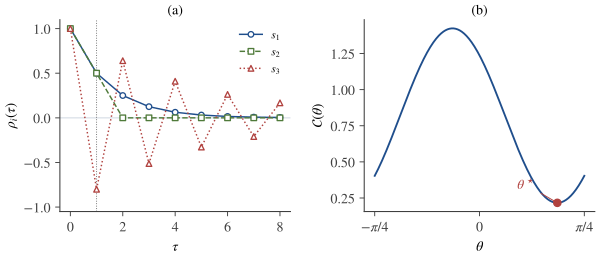
the real case of the formula of Cardoso and Souloumiac (1996), whose version also covers complex matrices. For a single matrix it reduces to the classical Jacobi angle $\tan2\theta = \beta/\alpha = 2[\bQ]_{pq}/([\bQ]_{pp} - [\bQ]_{qq})$ (Exercise 9.4习题 9.4). Each rotation minimizes $\mathcal{C}$ exactly over its plane, so $\mathcal{C}$ never increases. We compared (9.3) with a brute-force search over 20001 angles for 200 random sets of symmetric matrices: the closed form was never beaten, and the angles agreed to within the grid spacing. Figure 9.1图 9.1(b) shows the criterion of one pair as a function of $\theta$: a constant minus a sinusoid of period $\pi/2$, minimized at $\theta^\star$. In practice a few sweeps suffice. With exactly jointly diagonalizable matrices the decrease is very fast (in a test with $n = 6$ and $K = 5$, $\mathcal{C}$ went from 20 to $10^{-13}$ in three sweeps); with estimated matrices $\mathcal{C}$ levels off after two or three sweeps at a value set by the sampling error.

这是 Cardoso 与 Souloumiac（1996）公式的实数情形，他们的版本也适用于复矩阵。对单个矩阵，它退化为经典的 Jacobi 角 $\tan2\theta = \beta/\alpha = 2[\bQ]_{pq}/([\bQ]_{pp} - [\bQ]_{qq})$（Exercise 9.4习题 9.4）。每次旋转都在其所在平面内精确地最小化 $\mathcal{C}$，所以 $\mathcal{C}$ 从不增加。我们在 200 组随机对称矩阵上把 (9.3) 与对 20001 个角度的穷举搜索作了比较：闭式解从未被超越，两者给出的角度在网格间距以内一致。Figure 9.1图 9.1（b）画出了一对坐标的准则作为 $\theta$ 的函数：它是一个常数减去一个周期为 $\pi/2$ 的正弦曲线，在 $\theta^\star$ 处取最小值。实践中几次扫描就够了。对可以精确联合对角化的矩阵，下降非常快（在 $n = 6$、$K = 5$ 的测试中，$\mathcal{C}$ 在三次扫描内从 20 降到 $10^{-13}$）；对估计得到的矩阵，$\mathcal{C}$ 在两三次扫描后就稳定在由抽样误差决定的水平上。

9.4 JADEJADE 算法

JADE, for joint approximate diagonalization of eigenmatrices (Cardoso & Souloumiac, 1993), applies the Jacobi method to cumulant matrices. Let $\bQ_{kl} = \bQ_{\bz}(\be_k\be_l^\top)$, so that $[\bQ_{kl}]_{ij} = \cum(z_i, z_j, z_k, z_l)$; these $n^2$ matrices contain the whole cumulant tensor. The joint-diagonality criterion of this set is itself a function of the output cumulants.

JADE（joint approximate diagonalization of eigenmatrices，特征矩阵的联合近似对角化；Cardoso & Souloumiac, 1993）把 Jacobi 方法用于累积量矩阵。令 $\bQ_{kl} = \bQ_{\bz}(\be_k\be_l^\top)$，即 $[\bQ_{kl}]_{ij} = \cum(z_i, z_j, z_k, z_l)$；这 $n^2$ 个矩阵包含了整个累积量张量。这组矩阵的联合对角化准则本身就是输出累积量的函数。

The terms with $k = l = i$ in (9.4) form Comon's contrast $\sum_i\kurt(y_i)^2$ (Comon, 1994; Chapter 5第 5 章); JADE adds the cross-cumulants $\cum(y_i, y_i, y_k, y_l)$ with $(k, l) \ne (i, i)$. Both are maximized by the separating rotations; the extra terms are what turn the problem into joint diagonalization, with its closed-form Jacobi angles. Cardoso (1999) discusses the relations among these fourth-order contrasts. Two refinements make JADE practical. First, by part (c) of Proposition 9.1命题 9.1, the linear map $\bM \mapsto \bQ_{\bz}(\bM)$ has eigenpairs $(\lambda_r, \bM_r)$, and the left side of (9.4) equals $\sum_r\lambda_r^2\,\|\diag(\bU\bM_r\bU^\top)\|^2$ (Exercise 9.5习题 9.5). In the model only $n$ eigenvalues are nonzero, so JADE jointly diagonalizes the $n$ weighted eigenmatrices $\lambda_r\bM_r$ with the largest $|\lambda_r|$ instead of $n^2$ matrices; this is the "eigenmatrices" of its name. Second, the Jacobi updates touch only two rows and two columns of each matrix.

(9.4) 中 $k = l = i$ 的项构成 Comon 的对比函数 $\sum_i\kurt(y_i)^2$（Comon, 1994；Chapter 5第 5 章）；JADE 另外加上了 $(k, l) \ne (i, i)$ 的交叉累积量 $\cum(y_i, y_i, y_k, y_l)$。两者都在分离旋转处取最大值；正是这些额外的项把问题变成了联合对角化，从而可以使用闭式的 Jacobi 角。Cardoso（1999）讨论了这些四阶对比函数之间的关系。有两点改进使 JADE 实用。第一，由Proposition 9.1命题 9.1的（c），线性映射 $\bM \mapsto \bQ_{\bz}(\bM)$ 有特征对 $(\lambda_r, \bM_r)$，而 (9.4) 的左边等于 $\sum_r\lambda_r^2\,\|\diag(\bU\bM_r\bU^\top)\|^2$（Exercise 9.5习题 9.5）。在模型中只有 $n$ 个特征值非零，所以 JADE 只需联合对角化 $|\lambda_r|$ 最大的 $n$ 个加权特征矩阵 $\lambda_r\bM_r$，而不是 $n^2$ 个矩阵；这就是其名称中“特征矩阵”的由来。第二，Jacobi 更新每次只涉及每个矩阵的两行两列。

The following implementation favours clarity: it forms the full cumulant tensor with einsum, uses all $n^2$ matrices $\bQ_{kl}$, and rotates whole matrices. It is applied to a uniform, a Laplace and a binary source.

下面的实现以清晰为先：它用 einsum 构造完整的累积量张量，使用全部 $n^2$ 个矩阵 $\bQ_{kl}$，并对整个矩阵作旋转。示例中的源为一个均匀源、一个拉普拉斯源和一个二值源。

import numpy as np

def whiten(X):
    """Center the rows of X; return Z = V X (identity sample covariance) and V."""
    X = X - X.mean(axis=1, keepdims=True)
    d, E = np.linalg.eigh(np.cov(X))
    V = E @ np.diag(d ** -0.5) @ E.T
    return V @ X, V

def joint_diagonalize(Qs, tol=1e-12, max_sweeps=100):
    """Jacobi joint diagonalization of symmetric matrices Qs (shape K x n x n).
    Returns an orthogonal U that makes every U Q U^T as diagonal as possible."""
    Qs = Qs.copy()
    n = Qs.shape[1]
    U = np.eye(n)
    for sweep in range(max_sweeps):
        rotated = False
        for p in range(n - 1):
            for q in range(p + 1, n):
                h1 = Qs[:, p, p] - Qs[:, q, q]
                h2 = 2 * Qs[:, p, q]
                # closed-form Jacobi angle for the pair (p, q)
                theta = 0.25 * np.arctan2(2 * h1 @ h2, h1 @ h1 - h2 @ h2)
                if abs(theta) > tol:
                    rotated = True
                    c, s = np.cos(theta), np.sin(theta)
                    R = np.eye(n)
                    R[p, p] = R[q, q] = c
                    R[p, q], R[q, p] = -s, s
                    Qs = R.T @ Qs @ R      # rotate all matrices in the (p, q) plane
                    U = R.T @ U
        if not rotated:
            break
    return U

def jade(X):
    Z, V = whiten(X)
    n, T = Z.shape
    I = np.eye(n)
    M4 = np.einsum('it,jt,kt,lt->ijkl', Z, Z, Z, Z, optimize=True) / T
    C = (M4 - np.einsum('ij,kl->ijkl', I, I) - np.einsum('ik,jl->ijkl', I, I)
            - np.einsum('il,jk->ijkl', I, I))    # cumulant tensor of z
    Qs = C.reshape(n, n, n * n).transpose(2, 0, 1)    # the n^2 matrices Q(e_k e_l^T)
    return joint_diagonalize(Qs) @ V

rng = np.random.default_rng(1)
T = 10000
S = np.vstack([rng.uniform(-np.sqrt(3), np.sqrt(3), T),    # kappa = -1.2
               rng.laplace(0, 1 / np.sqrt(2), T),           # kappa = 3
               np.sign(rng.standard_normal(T))])            # kappa = -2
A = rng.standard_normal((3, 3))
P = jade(A @ S) @ A
print(np.round(P / np.abs(P).max(axis=1, keepdims=True), 2) + 0.0)

The printed global matrix, each row scaled by its largest entry, is a signed permutation up to entries of at most 0.03:

打印出的全局矩阵（每行除以该行绝对值最大的元素）在至多 0.03 的误差内是一个带符号的置换矩阵：

[[ 0.    0.03 -1.  ]
 [ 0.   -1.   -0.03]
 [-1.   -0.01  0.01]]

JADE needs no initialization and no step size, and its Jacobi sweeps are deterministic and few; its weakness is cost. Storing the $n^2$ cumulant matrices takes $n^4$ numbers ($6.25 \times 10^6$ for $n = 50$, $10^8$ for $n = 100$), and estimating them takes of the order of $n^4T$ operations. This restricts JADE to moderate numbers of sources, a few tens rather than hundreds.

JADE 不需要初始化，也没有步长，其 Jacobi 扫描是确定性的，次数也很少；它的弱点在于计算量。存储 $n^2$ 个累积量矩阵需要 $n^4$ 个数（$n = 50$ 时为 $6.25 \times 10^6$，$n = 100$ 时为 $10^8$），估计它们需要 $n^4T$ 量级的运算。这使 JADE 只适用于中等数目的源，即几十个而不是几百个。

9.5 Second-order methods: AMUSE and SOBI二阶方法：AMUSE 与 SOBI

The i.i.d. assumption of Assumption 1.1假设 1.1 discards the order of the samples. Many signals, from EEG rhythms to fMRI time courses, are correlated in time, and this structure can replace non-Gaussianity. Assume that the sources are zero-mean, wide-sense stationary, and mutually uncorrelated at every lag: $\E[s_i(t)s_j(t + \tau)] = 0$ for $i \ne j$ and all $\tau$. Write $\rho_i(\tau) = \E[s_i(t)s_i(t + \tau)]$ for the autocovariance of source $i$, with $\rho_i(0) = 1$. The lagged covariance matrices of the data are then

Assumption 1.1假设 1.1中的独立同分布假设丢弃了样本的顺序。许多信号，从 EEG 节律到 fMRI 时间过程，在时间上都是相关的，这种结构可以取代非高斯性。假设各源均值为零、宽平稳，并且在任何时滞下互不相关：对 $i \ne j$ 和所有 $\tau$ 有 $\E[s_i(t)s_j(t + \tau)] = 0$。记 $\rho_i(\tau) = \E[s_i(t)s_i(t + \tau)]$ 为源 $i$ 的自协方差，$\rho_i(0) = 1$。于是数据的时滞协方差矩阵为

They are symmetric in the model, but their estimates $\hat\bC_{\bx}(\tau) = \frac{1}{T - \tau}\sum_t\bx(t)\bx(t + \tau)^\top$ are not, so one uses $\bar\bC(\tau) = \tfrac12(\hat\bC(\tau) + \hat\bC(\tau)^\top)$. Whitening with $\bC_{\bx}(0) = \bA\bA^\top$ gives $\bar\bC_{\bz}(\tau) = \tilde\bA\,\diag(\rho_i(\tau))\,\tilde\bA^\top$ for every lag: again the joint diagonalization structure. Only second-order statistics are involved, so neither non-Gaussianity nor full independence is required.

在模型中这些矩阵是对称的，但其估计 $\hat\bC_{\bx}(\tau) = \frac{1}{T - \tau}\sum_t\bx(t)\bx(t + \tau)^\top$ 并不对称，所以使用 $\bar\bC(\tau) = \tfrac12(\hat\bC(\tau) + \hat\bC(\tau)^\top)$。用 $\bC_{\bx}(0) = \bA\bA^\top$ 白化后，对每个时滞都有 $\bar\bC_{\bz}(\tau) = \tilde\bA\,\diag(\rho_i(\tau))\,\tilde\bA^\top$：又是联合对角化的结构。这里只涉及二阶统计量，所以既不需要非高斯性，也不需要完全独立。

AMUSE. The AMUSE algorithm of Tong et al. (1990) uses a single lag: whiten, then take the eigenvectors of $\bar\bC_{\bz}(\tau)$. By Lemma 9.2引理 9.2 with $K = 1$, this separates the sources if and only if the numbers $\rho_1(\tau), \dots, \rho_n(\tau)$ are distinct; Tong et al. (1991) analyse the identifiability question in detail. Molgedey and Schuster (1994) proposed the same idea, formulated as the simultaneous diagonalization of $\bC_{\bx}(0)$ and $\bC_{\bx}(\tau)$. The condition is fragile: two sources with equal or nearly equal autocorrelation at the chosen lag are mixed, or estimated poorly, however different they are at other lags.

AMUSE。Tong 等（1990）提出的 AMUSE 算法只用一个时滞：先白化，再取 $\bar\bC_{\bz}(\tau)$ 的特征向量。由Lemma 9.2引理 9.2（取 $K = 1$），它能分离各源当且仅当 $\rho_1(\tau), \dots, \rho_n(\tau)$ 互不相同；Tong 等（1991）详细分析了其中的可辨识性问题。Molgedey 与 Schuster（1994）提出了同一思想，表述为 $\bC_{\bx}(0)$ 与 $\bC_{\bx}(\tau)$ 的同时对角化。这个条件是脆弱的：两个源若在所选时滞处自相关相等或接近相等，就会被混在一起或估计得很差，不管它们在其他时滞上相差多大。

This is SOBI, second-order blind identification (Belouchrani et al., 1997); TDSEP (Ziehe & Müller, 1998) is essentially the same method. Its identifiability condition follows directly from Lemma 9.2引理 9.2.

这就是 SOBI（second-order blind identification，二阶盲辨识；Belouchrani et al., 1997）；TDSEP（Ziehe & Müller, 1998）本质上是同一种方法。它的可辨识条件直接由Lemma 9.2引理 9.2得到。